1×9 adjoint(::Vector{Float64}) with eltype Float64:
0.0 0.375 0.75 1.125 1.5 1.875 2.25 2.625 3.0Machine Learning for Computational Economics
Module 02: Discrete-Time Methods
EDHEC Business School
January 2026
The Action-Value Function
The action-value function is given by \[ V_t(M, c) \equiv u(c) + e^{-\rho} \mathbb{E}\!\left[ V_{t-1}(R (M- c) + Y') \right]. \]
Tip
The action-value function corresponds to the value associated with a given action (no maximization step).
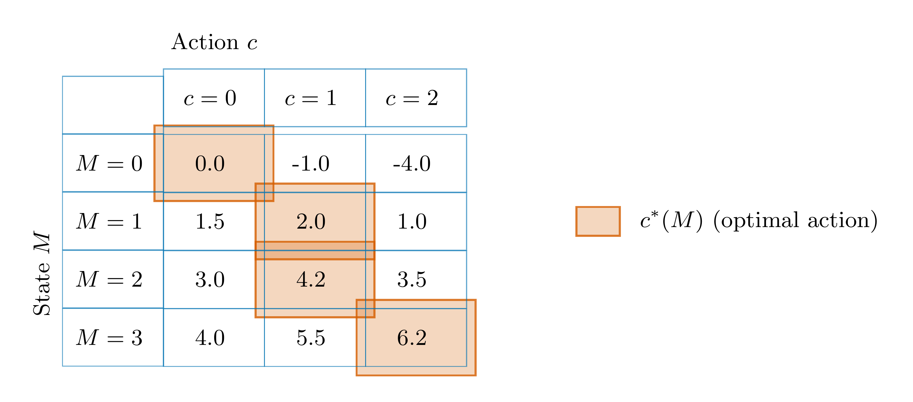
Think of \(V_t(M,c)\) as a table
- Columns: actions \(c\)
- Rows: states \(M\)
Optimal consumption: \[c_t(M) = \arg\max_{c} V_t(M,c)\]
Accuracy of a Linear Interpolation
The accuracy of a linear interpolation depends on the grid size.
- We can approximate even very non-linear functions this way.
- Depending on the function, this may require a very fine grid.
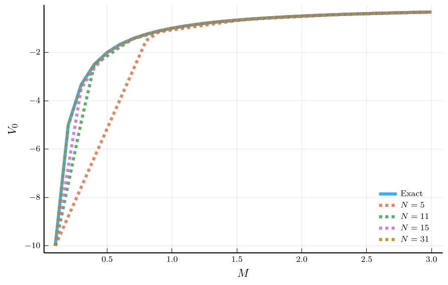
Quality of approximation may not be uniform
- Worse approximation near the boundaries.
Uniform grid can be very inefficient
- It does not allow to focus where it is needed
Non-Uniform Grids
An alternative is to use a non-uniform grid for the state variable.
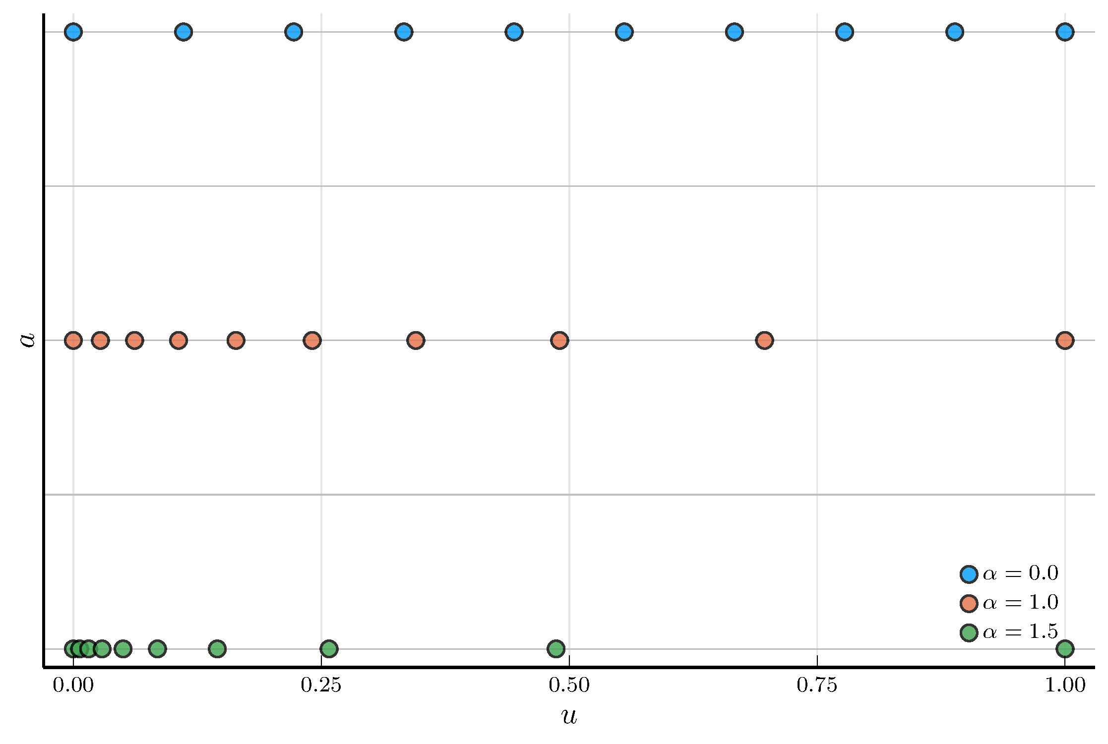
A convenient choice is the double-exponential grid
- Clusters grid points near the lower bound.
- Let \(u^j\) denote a uniform grid on the unit interval \([0,1]\).
- Define the grid points as \[ a_j = a_{\min} + (a_{\max} - a_{\min}) \frac{e^{\,e^{\alpha u^j}-1} - 1}{e^{\,e^{\alpha}-1} - 1}, \]
The parameter \(\alpha > 0\) controls the degree of clustering.
- As \(\alpha \to 0\), the grid becomes approximately uniform.
- For large \(\alpha\), the grid is very dense near the lower bound.
We can implement this in Julia as follows:
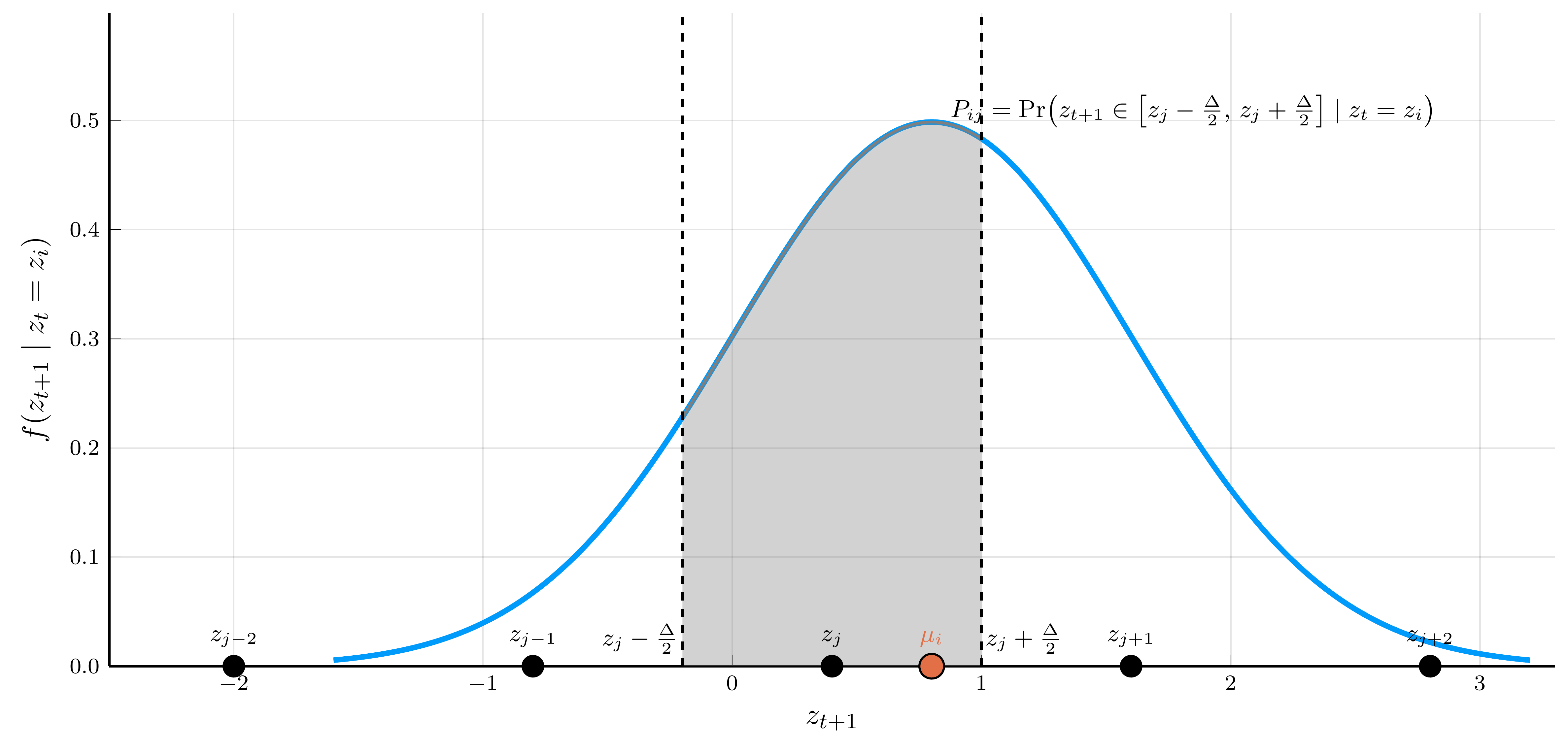
The Tauchen Method: Computing the Transition Probabilities
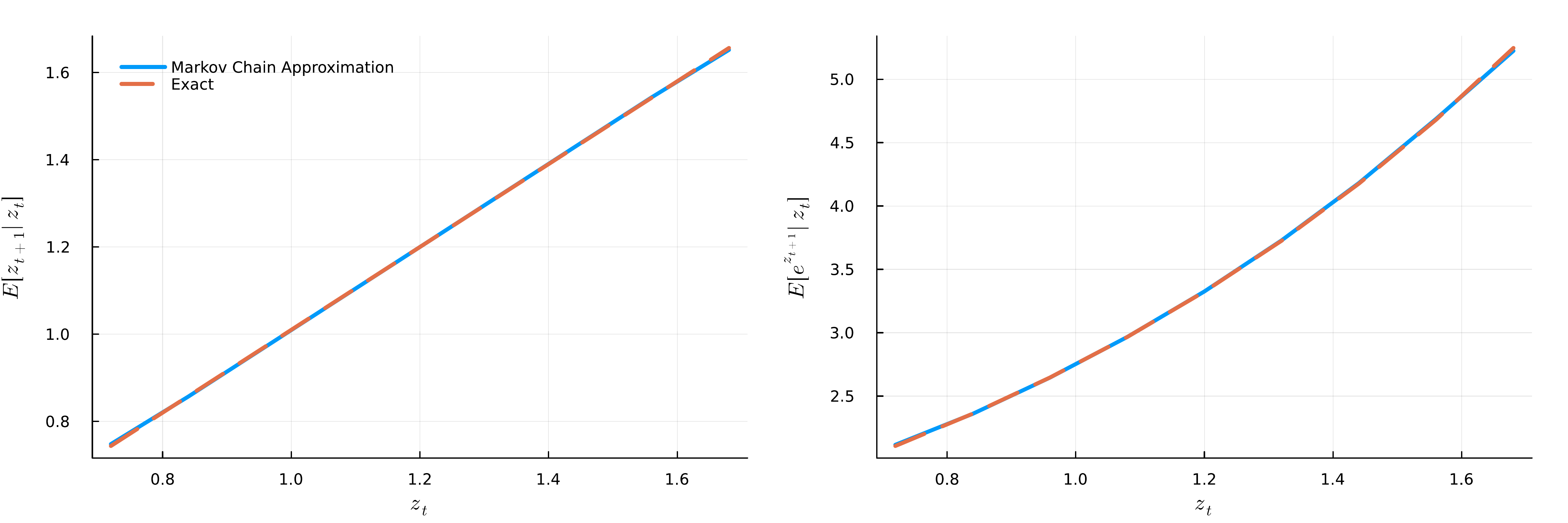
We need to determine the transition probabilities \(P_{ij} = \Pr(z_{t+1} = z_j \mid z_t = z_i)\).
- Conditional on \(z_t = z_i\), we have that \(z_{t+1} \sim \mathcal{N}\left(\mu + \rho_z (z_i - \mu), \sigma_\varepsilon^2\right)\).
The transition probability \(P_{ij}\) equals the probability that \(z_{t+1}\) falls between the midpoints surrounding \(z_j\):
\[\scriptsize P_{ij} = \begin{cases} \Phi\!\left(\dfrac{z_j - \mu_i + \tfrac{\Delta}{2}}{\sigma_\varepsilon}\right), & j = 1, \\[0.75em] \Phi\!\left(\dfrac{z_j - \mu_i + \tfrac{\Delta}{2}}{\sigma_\varepsilon}\right) - \Phi\!\left(\dfrac{z_j - \mu_i - \tfrac{\Delta}{2}}{\sigma_\varepsilon}\right), & 1 < j < N_z, \\[0.75em] 1 - \Phi\!\left(\dfrac{z_j - \mu_i - \tfrac{\Delta}{2}}{\sigma_\varepsilon}\right), & j = N_z, \end{cases} \]
Conditional Moments: Exact vs. Markov Chain Approximation
Policy and Value Functions
Two theoretical bounds for the policy function:
Lower bound: household receives the lowest income with certainty.
Upper bound: household receives the average income with certainty.

a) Policy functions
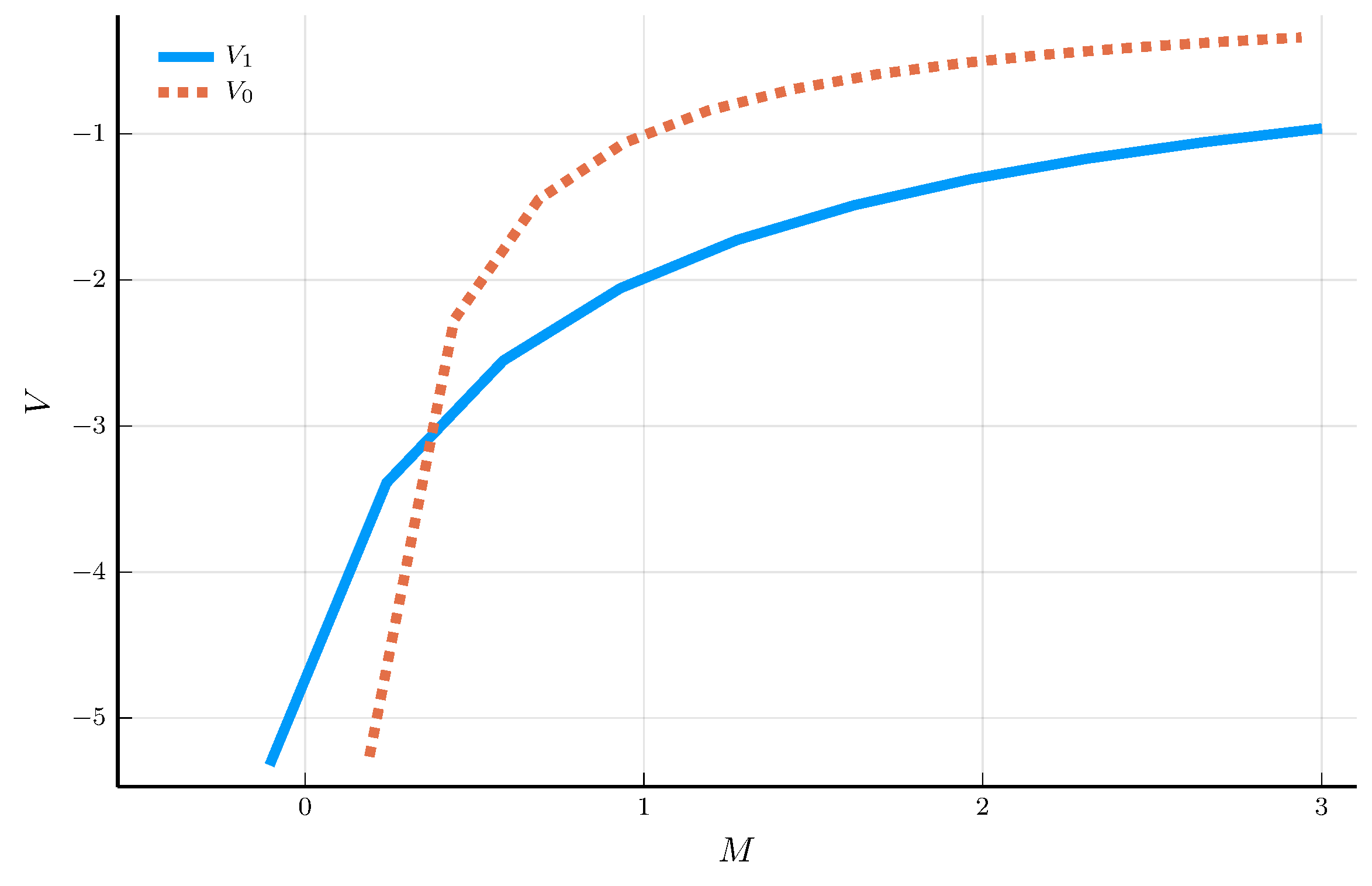
b) Value functions
The Marginal Propensity to Consume
Given the policy function \(c_t(M)\), we can obtain the marginal propensity to consume (MPC).
- The MPC measures the change in consumption for a change in \(M\): \(MPC(M) = \frac{d c_t(M)}{d M}\).
Carroll and Kimball (1996) show that the MPC is decreasing in \(M\).
- But the numerical solution does not necessarily satisfy this property.
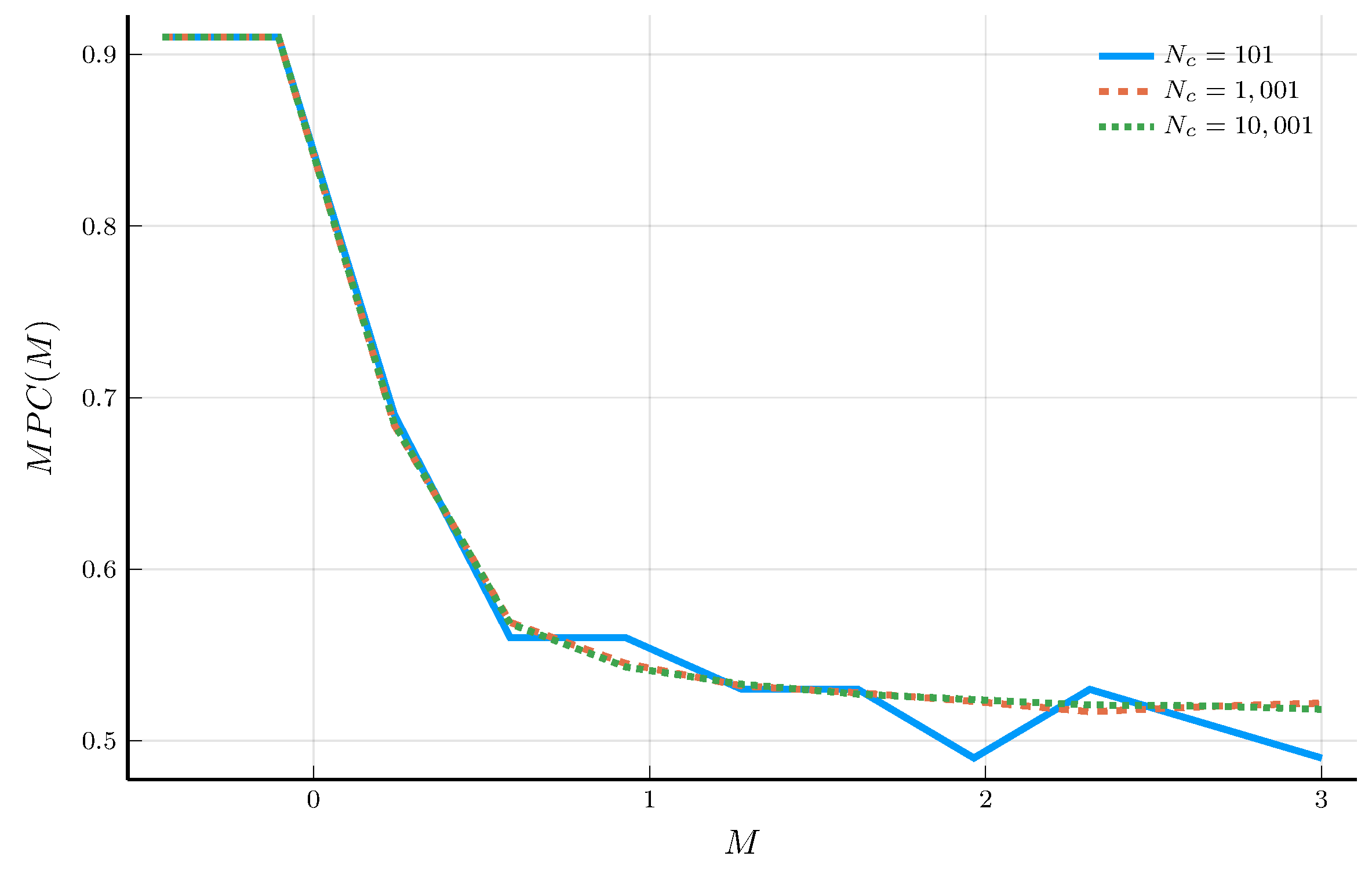
a) MPCs for \(N_M = 11\)
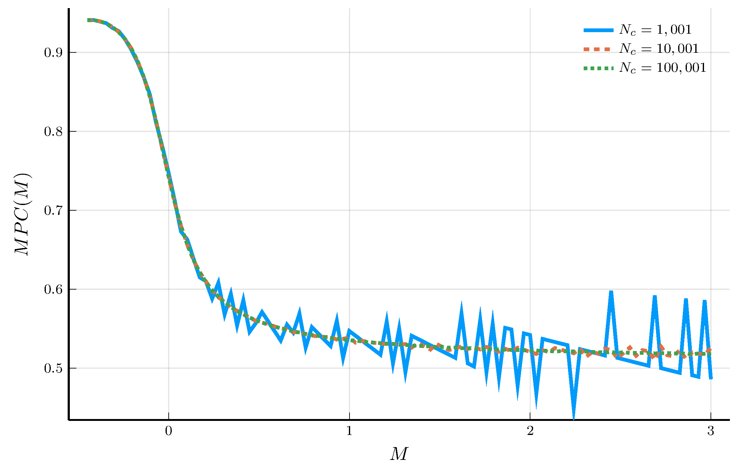
b) MPCs for \(N_M = 101\)
The EGM Iteration
We iterate the EGM step until the policy function converges.
We can compute the marginal propensity to consume (MPC) using the finite-difference method.
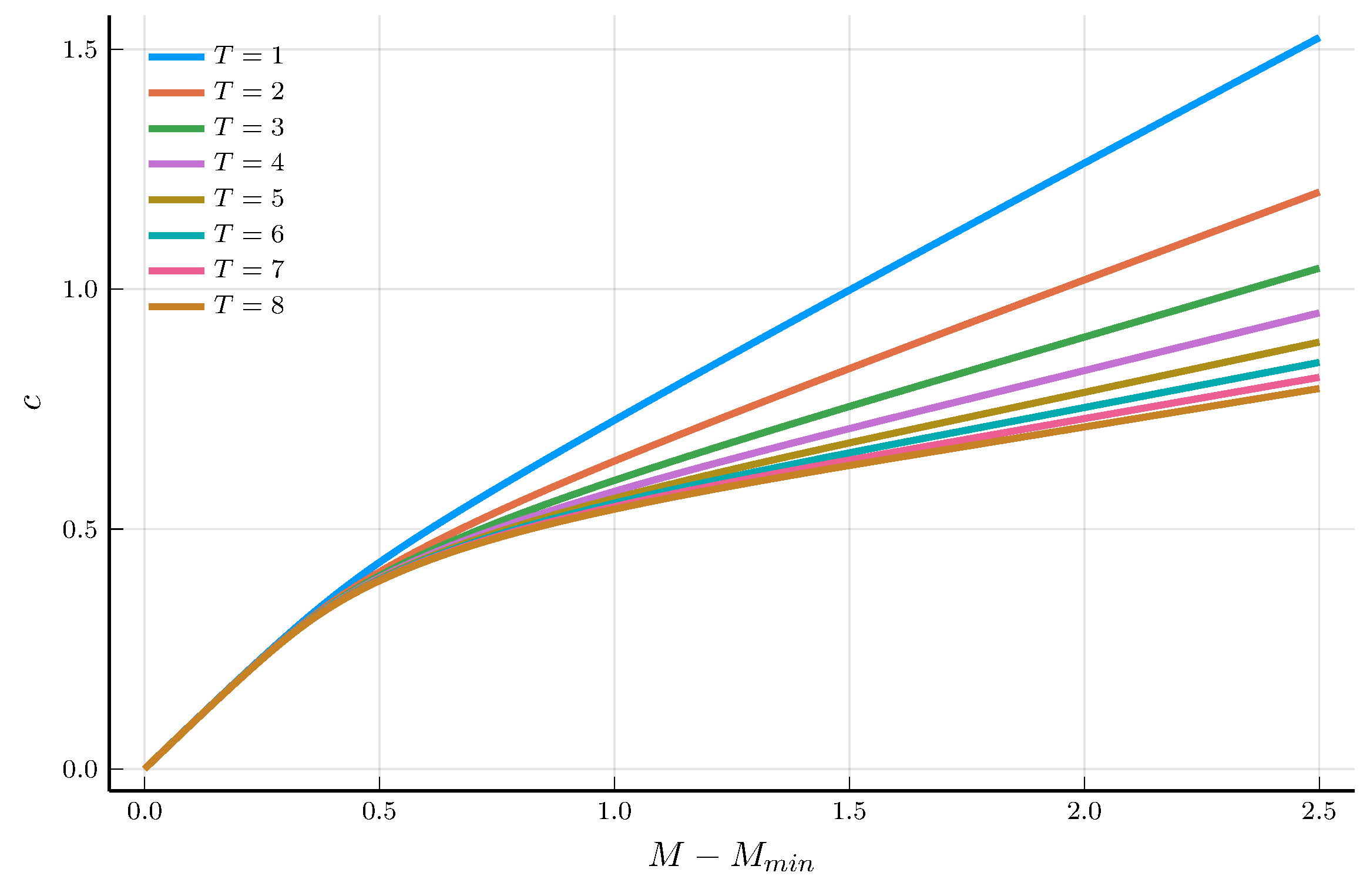
a) Policy function
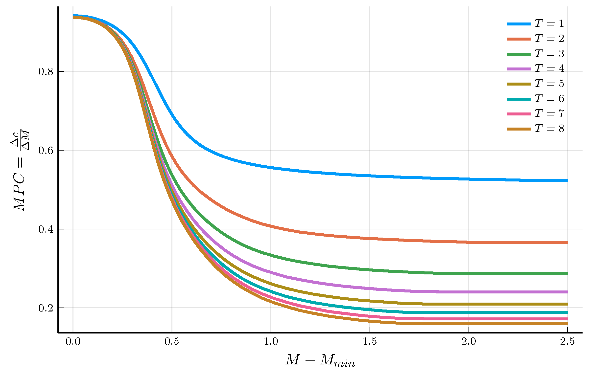
b) Marginal propensity to consume