Machine Learning for Computational Economics

Module 03: Continuous-Time Methods
EDHEC Business School

Dejanir Silva

Purdue University

January 2026

Introduction

Continuous-time formulations provide an elegant counterpart to discrete-time dynamic programming.

Instead of expectations over future states, they express optimal behavior through differential operators.
The solution is characterized by a partial differential equation (PDE).

In this module, we revisit the consumption-savings problem from Module 02.

We show how to derive the Hamilton-Jacobi-Bellman (HJB) equation.
We solve the HJB equation numerically using finite-difference schemes and spectral methods.

The module is organized as follows:

Derivation of the HJB equation.
Solution and stability of finite-difference schemes.
Application of spectral methods.

I. From Discrete to Continuous Time

A Portfolio Choice Problem with Uninsurable Income

We extend the consumption-savings problem from Module 02 in two dimensions:

The household faces a portfolio choice problem: she decides how much to save in a safe and a risky asset.
Labor income follows a persistent Markov process rather than being i.i.d. over time.

Asset returns:

Riskless return over a small interval \(\Delta t\) is \[ R_f = 1 + r\,\Delta t, \] and the return on the risky asset is: \[ R_{r,t+\Delta t} = 1 + \mu_r\,\Delta t + \sigma_r \sqrt{\Delta t}\,\varepsilon_{r,t+\Delta t}, \] where \(\varepsilon_{r,t+\Delta t}\) is a unit-variance white noise.

Labor income:

Labor income follows a (discrete-state) Markov chain: \[ Y_t \in \{Y_1, \ldots, Y_{N_y}\}, \] with transition probabilities \[ P_{ij} = \lambda_{ij}\,\Delta t, \qquad j \neq i, \] and \(P_{ii} = 1 - \sum_{j \neq i} P_{ij}\).

Note

The scaling ensures that mean and variance of the risky return are of order \(\Delta t\). To see this, fix a horizon \(T = n\,\Delta t\) and note that \[ \operatorname{Var}\!\left[\sum_{k=1}^{n} R_{r,t+k\Delta t}\right] = n\,\sigma_r^2\,\Delta t = \sigma_r^2\,T. \] Hence, as we partition the time interval into finer and finer subperiods, the total amount of risk over \([t,\,t+T]\) remains unchanged.

The Bellman Equation with Time Step \(\Delta t\)

The Bellman equation for this discrete-time formulation is \[ V_t(W, Y) = \max_{c, \alpha} \left\{ u(c)\,\Delta t + e^{-\rho \Delta t}\, \mathbb{E}\left[V_{t-\Delta t}(W', Y')\right] \right\}, \] subject to the law of motion for wealth, \[ W' = R_{p,t+\Delta t}\,\bigl(W + (Y - c)\,\Delta t\bigr), \qquad R_{p,t+\Delta t} = (1-\alpha)\,R_f + \alpha\,R_{r,t+\Delta t}, \] and a borrowing limit \(W \geq \underline{W}\), given a transition matrix \(\Pr(Y' = Y_j \mid Y = Y_i) = P_{ij}\).

Note

When deriving the continuous-time limit, it is essential to distinguish between flow and stock variables. The cash-on-hand variable, \[ M = W + Y\,\Delta t, \] combines a stock (wealth) with a flow (labor income). As \(\Delta t \to 0\), this distinction vanishes, and \(M\) and \(W\) coincide in the limit.

State Dynamics in Continuous Time

Wealth dynamics.

The discrete-time wealth process can be expressed as \[ W_{t+\Delta t} - W_t = [(1-\alpha_t) r W_t + \alpha_t \mu_r W_t + Y_t - c_t]\Delta t + \alpha_t \sigma_r W_t \sqrt{\Delta t}\,\varepsilon_{r,t+\Delta t} + o(\Delta t), \]

Taking the limit as \(\Delta t \to 0\), we obtain the continuous-time wealth dynamics: \[ dW_t = [(1-\alpha_t) r W_t + \alpha_t \mu_r W_t + Y_t - c_t] dt + \alpha_t \sigma_r W_t\, dB_t, \] where \(B_t\) is a standard Brownian motion.

Labor income dynamics.

The expected change in income over a small interval \(\Delta t\) is \[ \mathbb{E}\left[Y_{t+\Delta t} - Y_t \mid Y_t = Y_i\right] = \sum_{j \neq i} \lambda_{ij} (Y_j - Y_i)\,\Delta t. \] In continuous time, this implies the following jump process for income: \[ dY_t = \sum_{j} (Y_j - Y_i)\, dN_{ij,t}, \qquad \mathbb{E}[dN_{ij,t}] = \lambda_{ij}\,dt, \]

The Hamilton-Jacobi-Bellman Equation

We now derive the continuous-time version of the Bellman equation: \[ 0 = \max_{c, \alpha} \Big\{ u(c) + \frac{\mathbb{E}\!\left[V_{t-\Delta t}(W',Y') - V_t(W,Y)\,\middle|\,W,Y\right]}{\Delta t} - \rho\,V_t(W,Y) \Big\} + O(\Delta t). \] subject to the wealth dynamics and labor income dynamics.

Taking the limit as \(\Delta t \to 0\), we obtain the continuous-time Bellman equation: \[ \rho V_t(W,Y)\,dt = \max_{c, \alpha} \Big\{ u(c)\,dt + \color{#d55e00}{\underbrace{\mathbb{E}\!\left[dV_t(W,Y)\right]}_{\text{drift term}}} \Big\}. \]

Applying Itô’s lemma to \(V_t(W,Y)\), we obtain the Hamilton-Jacobi-Bellman (HJB) equation:

\[ \rho V_t(W,Y_i) = \max_{c,\alpha} \Big\{ u(c) - \frac{\partial V_t}{\partial t} + \mathcal{D}V_t(W,Y_i) + \sum_{j \neq i} \lambda_{ij}\big[V_t(W,Y_j) - V_t(W,Y_i)\big] \Big\}, \] where \(\mathcal{D}\) is the Dynkin operator: \[ \mathcal{D}V_t(W,Y) = V_W\,[r W + \alpha (\mu_r - r) W + Y - c_t] + \tfrac{1}{2} V_{WW}\,(\alpha \sigma_r W)^2. \]

II. Finite Differences: Black–Scholes–Merton

A Black–Scholes–Merton Example

We now show how to solve the HJB equation numerically using finite differences.

As a warm-up exercise, we consider an option pricing problem in the Black–Scholes–Merton framework.
This will provide a simpler setting where we can illustrate the main idea of the finite-difference method.

Asset dynamics:

The risk-free rate is constant and equal to \(r\),
The stock price follows a geometric Brownian motion: \[ dS_t = \mu_S S_t\,dt + \sigma_S S_t\,dB_t, \] where \(B_t\) is a standard Brownian motion.

No arbitrage:

We are interested in pricing the option using the principle of no-arbitrage.
The absence of arbitrage opportunities implies the existence of a stochastic discount factor \(\pi_t\): \[ d\pi_t = -r\,\pi_t\,dt - \eta\,\pi_t\,dB_t, \] where \(\eta \equiv \frac{\mu_S - r}{\sigma_S}\) is the market price of risk.

The Black–Scholes–Merton PDE

The value of a call option is given by \[ V_T(S) = \mathbb{E}_0\!\left[ \frac{\pi_T}{\pi_0}\,\max(S_T - K, 0) \,\middle|\, S_0 = S \right]. \] with terminal payoff \(V_T(S) = \max(S - K, 0)\).

The HJB equation for this problem at time \(t \geq 0\) is \[ 0 = \mathbb{E}_t\!\left[\, d \bigl(\pi_t\,V_{T-t}(S_t)\bigr) \right]. \]

Applying Itô’s lemma to \(\pi_t V_{T-t}(S_t)\), we obtain the Black–Scholes–Merton PDE: \[ -r\,V_T(S) - \frac{\partial V_T(S)}{\partial T} + r\,S\,\frac{\partial V_T(S)}{\partial S} + \tfrac{1}{2}\sigma_S^2 S^2\,\frac{\partial^2 V_T(S)}{\partial S^2} = 0, \] with terminal condition \(V_0(S) = \max(S - K, 0)\).

Tip

It is convenient to express the PDE in terms of the log stock price \(s \equiv \log S\): \[ -r\,v_T(s) - \frac{\partial v_T(s)}{\partial T} + \overline{r}\,\frac{\partial v_T(s)}{\partial s} + \frac{1}{2}\sigma_S^2\,\frac{\partial^2 v_T(s)}{\partial s^2} = 0, \] with terminal condition \(v_0(s) = \max(e^s - K, 0)\), where \(\overline{r} \equiv r - \tfrac{1}{2}\sigma_S^2\) is the risk-adjusted drift.

Finite-difference approximations

We can solve the PDE by discretizing both time and space (\(t\) and \(s\)).

Let \(t \in \{t_1, t_2, \ldots, t_M\}\) be the time on a uniform grid.
Let \(s \in \{s_1, s_2, \ldots, s_N\}\) be the log stock price on a uniform grid.

We can approximate the spatial derivatives in different ways:

Forward difference: \[ \frac{\partial v_{t_n}(s_i)}{\partial s} = \frac{v_{i+1}^n - v_i^n}{\Delta s}, \]

Backward difference: \[ \frac{\partial v_{t_n}(s_i)}{\partial s} = \frac{v_i^n - v_{i-1}^n}{\Delta s}, \]

Centered difference: \[ \frac{\partial v_{t_n}(s_i)}{\partial s} = \frac{v_{i+1}^n - v_{i-1}^n}{2\Delta s}. \]

The second spatial derivative is approximated by a centered difference: \[ \frac{\partial^2 v_{t_n}(s_i)}{\partial s^2} = \frac{v_{i+1}^n - 2v_i^n + v_{i-1}^n}{\Delta s^2}. \]

The time derivative is approximated by a forward Euler step: \[ \frac{\partial v_{t_n}(s_i)}{\partial T} = \frac{v_i^{n+1} - v_i^n}{\Delta t}. \]

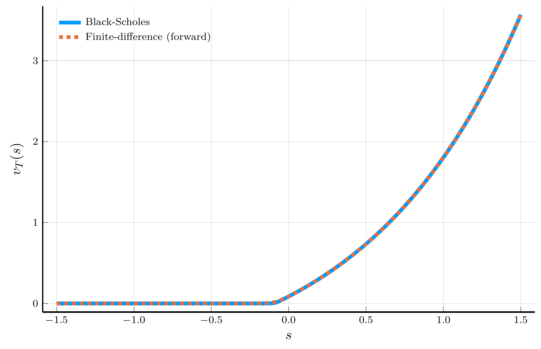
Explicit scheme

We fix a forward difference in time and consider two versions for the spatial derivative:

The forward-difference version is \[ r\,v_i^n = -\frac{v_i^{n+1} - v_i^n}{\Delta t} + \overline{r}\color{#d55e00}{\,\frac{v_{i+1}^n - v_i^n}{\Delta s}} + \frac{\sigma_S^2}{2}\,\frac{v_{i+1}^n - 2v_i^n + v_{i-1}^n}{\Delta s^2}, \]

The backward-difference version is \[ r\,v_i^n = -\frac{v_i^{n+1} - v_i^n}{\Delta t} + \overline{r}\color{#009e73}{\,\frac{v_i^n - v_{i-1}^n}{\Delta s}} + \frac{\sigma_S^2}{2}\,\frac{v_{i+1}^n - 2v_i^n + v_{i-1}^n}{\Delta s^2}. \]

Rearranging either form gives a common update rule: \[ v_i^{n+1} = -r\,\Delta t\,v_i^n + p_u\,v_{i+1}^n + p_s\,v_i^n + p_d\,v_{i-1}^n, \qquad i=2, \ldots, N-1, \] where, letting \(\mathbf{1}_{\text{F}}\) and \(\mathbf{1}_{\text{B}}\) denote the forward and backward difference indicators,

\[ p_u = \frac{\overline{r}\,\Delta t}{\Delta s}\,\mathbf{1}_{\text{F}} + \frac{\sigma_S^2\,\Delta t}{2\Delta s^2}, \qquad \qquad p_s = 1 - \frac{\overline{r}\,\Delta t}{\Delta s}\,(\mathbf{1}_{\text{F}} - \mathbf{1}_{\text{B}}) - \frac{\sigma_S^2\,\Delta t}{\Delta s^2}, \qquad \qquad p_d = -\frac{\overline{r}\,\Delta t}{\Delta s}\,\mathbf{1}_{\text{B}} + \frac{\sigma_S^2\,\Delta t}{2\Delta s^2}. \]

Boundary conditions

We handle boundaries using ghost nodes, i.e., values outside the grid.

Right boundary. Option is deep in the money, so \(\frac{\partial v_{t_n}(s_N)}{\partial s} = e^{s_N}\): \[ v_{N+1}^n = v_N^n + e^{s_N}\,\Delta s. \]

Left boundary. Option is far out of the money, so \(\frac{\partial v_{t_n}(s_1)}{\partial s} = 0\): \[ v_0^n = v_1^n. \]

Matrix representation

Define \(\mathbf{v}^n = [v_1^n, v_2^n, \ldots, v_N^n]^\top\) and the tridiagonal matrix of coefficients: \[ \mathbf{P} = \begin{pmatrix} p_s + p_d & p_u & 0 & \ldots & 0 \\ p_d & p_s & p_u & \ldots & 0 \\ \vdots & \vdots & \vdots & \ddots & \vdots \\ 0 & \ldots & p_d & p_s & p_u \\ 0 & \ldots & 0 & p_d & p_s + p_u \end{pmatrix}. \] Then the law of motion for \(\mathbf{v}^n\) is \[ \mathbf{v}^{n+1} = \mathbf{P}^r\,\mathbf{v}^n + \mathbf{b}, \qquad \mathbf{P}^r \equiv \mathbf{P} - r\,\Delta t\,\mathbf{I}_N, \] with initial condition \(\mathbf{v}^0 = [v_0(s_1), v_0(s_2), \ldots, v_0(s_N)]^\top\), and adjustment vector \(\mathbf{b} = [0, \ldots, 0,\, p_u\,e^{s_N}\,\Delta s]^\top\).

Julia implementation

We start by defining the model structure for the Black–Scholes–Merton problem.

@kwdef struct BlackScholesModel
    σS::Float64 = 0.20
    r::Float64 = 0.05
    K::Float64 = 1.0
    T::Float64 = 1.0
    Ns::Int64 = 150
    Nt::Int64 = 300
    sgrid::LinRange{Float64} = range(-1.5, 1.5, length=Ns)
end

We then implement the finite-difference scheme.

function fd_scheme(m::BlackScholesModel; forward::Bool = true)
    (; σS, r, K, T, Ns, Nt, sgrid) = m # unpack model parameters
    Δs, Δt = sgrid[2] - sgrid[1], T / (Nt - 1) # spatial/time steps
    r̅ = r - 0.5 * σS^2 # risk-adjusted drift
    # Coefficients for the tridiagonal matrix
    pu = r̅ * Δt / Δs * forward + σS^2 * Δt / (2 * Δs^2)
    ps = 1 - r̅ * Δt / Δs * (2*forward-1) - σS^2 * Δt / (Δs^2)
    pd = -r̅ * Δt / Δs * (1-forward) + σS^2 * Δt / (2 * Δs^2)
    e  = zeros(Ns)
    e[1], e[end] = pd, pu # set boundary conditions
    P = Tridiagonal(pd*ones(Ns-1), ps*ones(Ns)+e, pu*ones(Ns-1))
    # Boundary conditions
    b = zeros(Ns)
    b[end] = pu * exp(sgrid[end]) * Δs
    # Initial condition
    v = @. max(0.0, exp(sgrid) - K) # terminal condition
    for n in 2:Nt
        v = (P - r * Δt * I) * v + b # update rule
    end
    return (; P, b, v)
end

Forward vs. Backward Differences

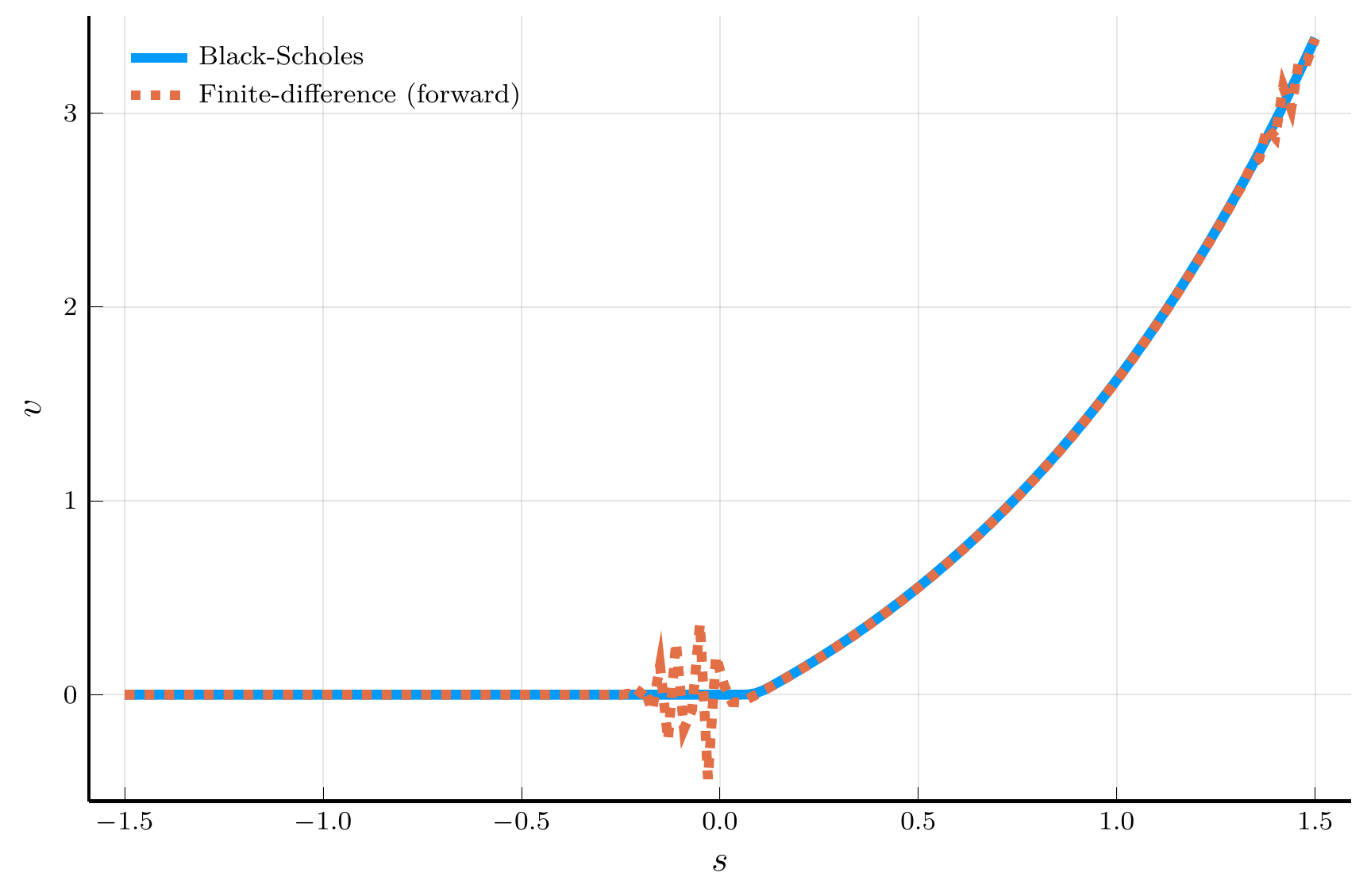
Forward difference

Backward difference

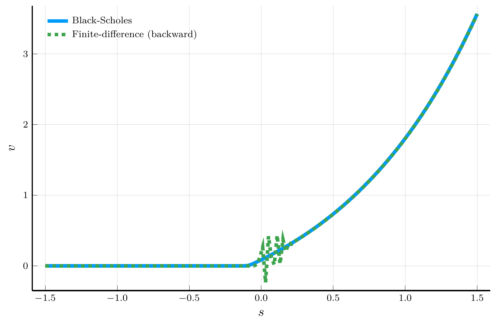
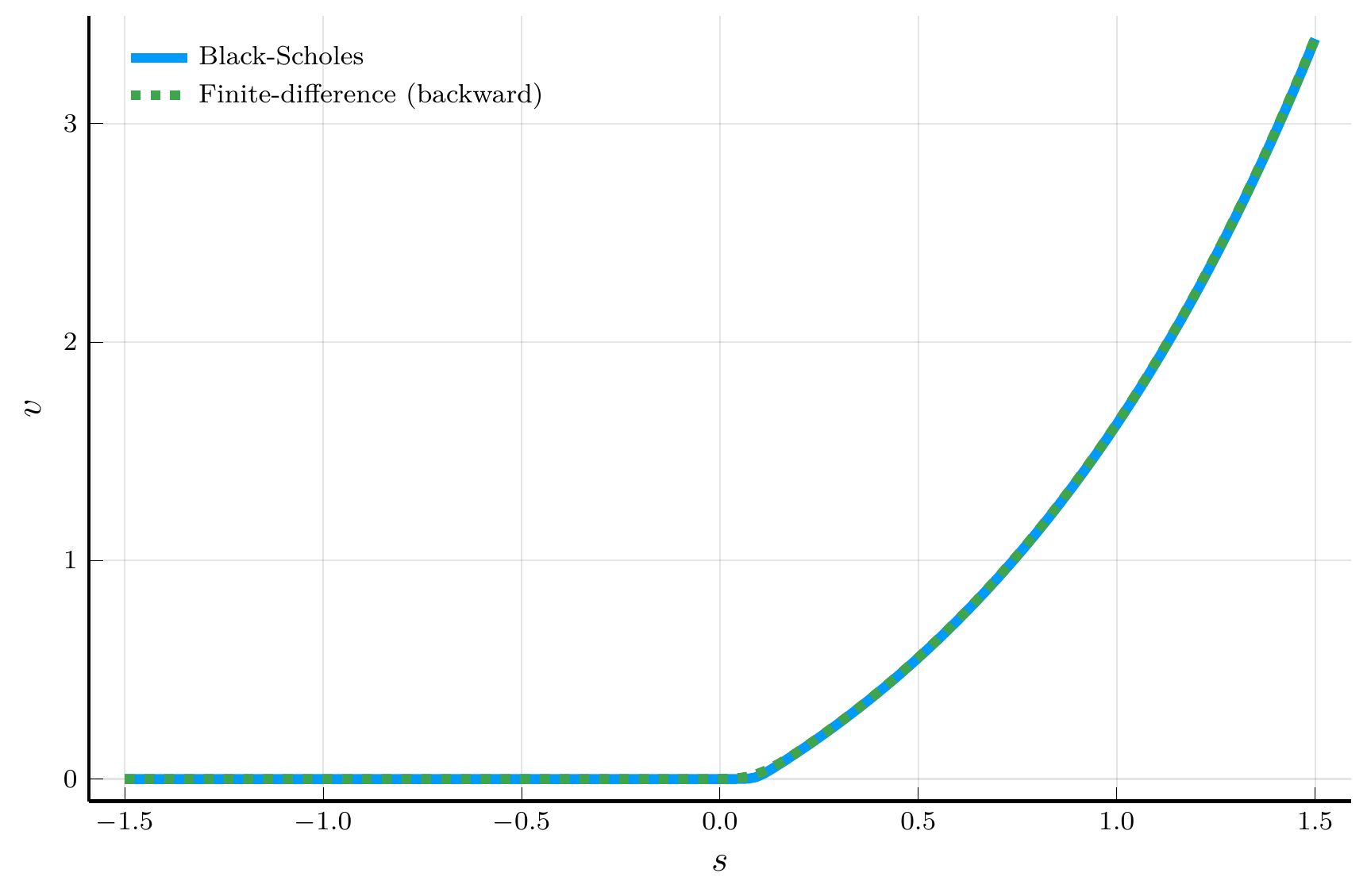
Top row: positive drift. Bottom row: negative drift.

Markov Chain Approximation (MCA)

The plots above motivate the use of an upwind scheme:

Use a forward difference when the drift is positive.
Use a backward difference when the drift is negative.

This choice suppresses numerical oscillations and improves stability of the explicit scheme.

But why does upwinding work?

A useful perspective comes from the Markov Chain Approximation (MCA) of Kushner and Dupuis (2001).

The MCA approach starts from the discretized Bellman equation \[ v_T(s) = (1 - r\,\Delta t)\,\mathbb{E}\!\left[\,v_{T-\Delta t}(s') \,\middle|\, s\,\right], \] under the risk–neutral log–price dynamics with drift \(\overline r\) and variance \(\sigma_S^2\): \[ \mathbb{E}[\,s' - s \mid s\,] = \overline r\,\Delta t, \qquad \operatorname{Var}[\,s' \mid s\,] = \sigma_S^2\,\Delta t. \]

Key idea: Let’s assume \(s\) follows a Markov chain on the grid \(\{s_i\}_{i=1}^N\)

Starting at \(s_i\), the log price can move only to \(s_{i-1}\), \(s_i\), or \(s_{i+1}\)
The transition probabilities \((p_d, p_s, p_u)\) are chosen to match the local mean and variance.

The CFL Condition

A locally consistent choice for the transition probabilities is \[ p_u = \frac{\overline r\,\Delta t}{\Delta s}\,\mathbf{1}_{\{\overline r \ge 0\}} + \frac{\sigma_S^2\,\Delta t}{2\Delta s^2},\quad p_s = 1 - \frac{|\overline r|\,\Delta t}{\Delta s} - \frac{\sigma_S^2\,\Delta t}{\Delta s^2},\quad p_d = -\,\frac{\overline r\,\Delta t}{\Delta s}\,\mathbf{1}_{\{\overline r < 0\}} + \frac{\sigma_S^2\,\Delta t}{2\Delta s^2}. \]

We need to ensure that \((p_d, p_s, p_u)\) are non-negative and sum to 1.

These satisfy \(p_u + p_s + p_d = 1\) by construction.
Upwinding ensures \(p_u \ge 0\) and \(p_d \ge 0\)

To ensure the nonnegativity of \(p_s\), we need to impose the Courant–Friedrichs–Lewy (CFL) condition: \[ 1 - \frac{|\overline r|\,\Delta t}{\Delta s} - \frac{\sigma_S^2\,\Delta t}{\Delta s^2} \ge 0 \quad\Longleftrightarrow\quad \Delta t \le \frac{\Delta s^2}{\,|\overline r|\,\Delta s + \sigma_S^2\,}. \]

Important

The CFL condition is crucial to ensure that the transition probabilities are non-negative.

Violating it produces instability and spurious oscillations in the numerical solution.

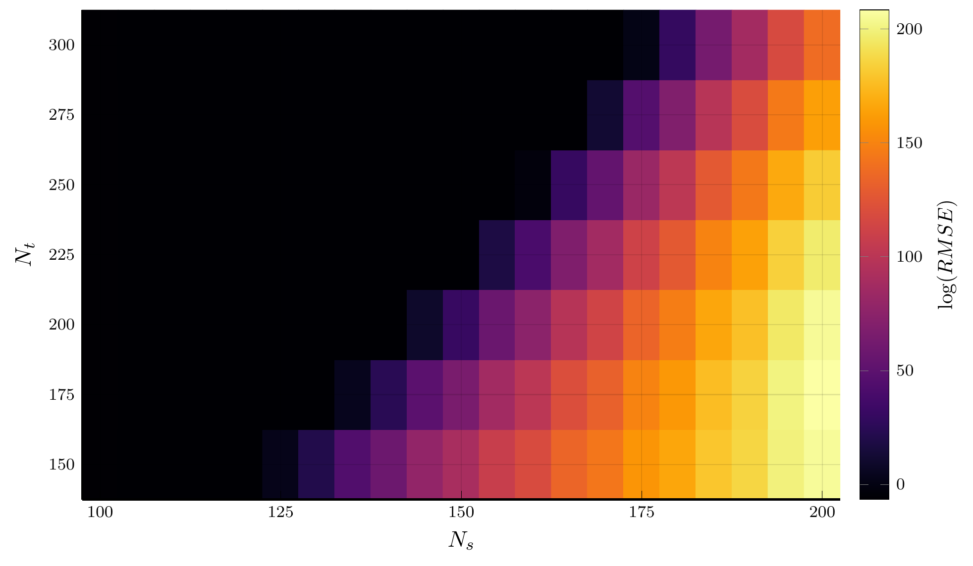
Discretization Error

A key aspect of the CFL condition for the explicit scheme is a restriction on \(\Delta t\)

The time step \(\Delta t\) must shrink as the spatial step \(\Delta s\) shrinks to maintain stability.
We can illustrate this with a heatmap of the discretization error.

The Barles-Souganidis Conditions

The analysis above provided a probabilistic intuition for the stability of the finite-difference scheme.

A complementary and more general approach is given by the Barles and Souganidis (1991) theorem.
The theorem provides sufficient conditions for the convergence of the finite-difference schemes

Main result. Consider a numerical scheme of the general form \[ F^h(x, V(x), V(\cdot)) = 0, \] where \(h\) collects the discretization parameters (e.g., \(\Delta t\), \(\Delta s\)), and \(V\) is the numerical approximation to the value function.

Barles and Souganidis (1991) provide conditions for the convergence to the viscosity solution of the HJB equation.

Barles–Souganidis theorem

Suppose that the continuous-time problem admits a unique bounded viscosity solution. If a numerical scheme is:

Monotone: The numerical operator \(F^h\) is non-decreasing in \(V\).
Stable: The sequence of numerical approximations \(V^h\) remains uniformly bounded.
Consistent: As \(h \to 0\), the discrete operator \(F^h\) converges to the continuous operator \(F\) defining the PDE.

Then the scheme converges locally uniformly to the viscosity solution of the HJB equation.

Tip

A viscosity solution is a generalized notion of solution to nonlinear PDEs like the HJB equation, which applies to problems where the value function may exhibit kinks or corners, as is typical in dynamic optimization problems with borrowing constraints or nonconvexities.

Connection to the explicit upwind scheme

Consider our explicit upwind scheme: \[ v_i^{n+1} = p_u^r\,v_{i+1}^n + p_s^r\,v_i^n + p_d^r\,v_{i-1}^n + b_i^n, \] with coefficients \(p_u^r = p_u, p_s^r = p_s-r\,\Delta t, p_d^r = p_d\).

The scheme is therefore:

Monotone: if \(p_u^r, p_s^r, p_d^r \ge 0\) — that is, when upwinding and the CFL condition hold.
Stable: if \(\|v^n\|\) remains bounded, which again follows from \(p_u^r + p_s^r + p_d^r = 1-r\,\Delta t \leq 1\) and nonnegativity.
Consistent: because the finite-difference approximations converge to their continuous counterparts as \(\Delta s, \Delta t \to 0\).

Implicit schemes

We will use the Barles–Souganidis theorem to analyze the stability of implicit schemes.

The implicit version of the discretization of the Black–Scholes–Merton PDE is \[ r\,v_i^{n+1} = -\frac{v_i^{n+1} - v_i^n}{\Delta t} + \overline{r} \left[\mathbf{1}_{\{\overline{r} \ge 0\}} \,\frac{v_{i+1}^{n+1} - v_i^{n+1}}{\Delta s} + \mathbf{1}_{\{\overline{r} < 0\}} \,\frac{v_{i}^{n+1} - v_{i-1}^{n+1}}{\Delta s}\right] + \frac{\sigma_S^2}{2}\,\frac{v_{i+1}^{n+1} - 2v_i^{n+1} + v_{i-1}^{n+1}}{\Delta s^2}, \]

We can rewrite the equation above as \[ v_i^{n+1} = v_i^n + p_u^r\,v_{i+1}^{n+1} - \delta^r\,v_i^{n+1} + p_d^r\,v_{i-1}^{n+1}, \] where \(\delta^r \equiv p_u^r+p_d^r+r\,\Delta t\).

In matrix form, we have \[ \mathbf{A} \mathbf{v}^{n+1} = \mathbf{v}^n+ \mathbf{b}, \] where \(\mathbf{A}\) is a tridiagonal matrix of coefficients: \[ \mathbf{A} = \begin{pmatrix} 1+\delta^r - p_d^r &-p_u^r & 0 & \ldots & 0 \\ -p_d^r & 1+\delta^r & -p_u^r & \ldots & 0 \\ \vdots & \vdots & \vdots & \ddots & \vdots \\ 0 & \ldots & -p_d^r & 1+\delta^r & -p_u^r \\ 0 & \ldots & 0 & -p_d^r & 1+\delta^r -p_u^r \end{pmatrix}. \]

Checking the Barles-Souganidis conditions

We need to check that the scheme is monotone, stable, and consistent.

The discretization ensures consistency and \(r>0\) ensures stability.
The main condition we need to check is monotonicity.
Monotonicity requires that, if \(\mathbf{v}^n\) and \(\mathbf{u}^{n}\) satisfy the recursion, and \(\mathbf{v}^n \ge \mathbf{u}^{n}\), then \(\mathbf{v}^{n+1} \ge \mathbf{u}^{n+1}\).

This is equivalent to saying that \(\mathbf{A}\) is a M-matrix.🌐

Sufficient condition: off-diagonal elements are non-positive and the diagonal is strictly dominant: \(\mathbf{A}_{ii} > \sum_{j \neq i} |\mathbf{A}_{ij}|\).
Upwinding ensures that the off-diagonal elements, \(p_u^r\) and \(p_d^r\), are non-positive.

Strict diagonal dominance requires: \[ 1+\delta^r > |p_d^r| + |p_u^r| \iff 1+r \Delta t > 0, \] which holds for any \(\Delta t > 0\) provided \(r > 0\).

Important

The condition above plays the same role as the CFL condition in ensuring monotonicity, but unlike in the explicit scheme, it imposes no restriction on \(\Delta t\). This property is often referred to as unconditional stability.

Julia implementation

We can implement the implicit scheme as follows:

function fd_implicit(m::BlackScholesModel)
    (; σS, r, K, T, Ns, Nt, sgrid) = m # unpack model parameters
    Δs, Δt = sgrid[2] - sgrid[1], T / (Nt - 1) # spatial/time steps
    r̅ = r - 0.5 * σS^2 # risk-adjusted drift
    # Coefficients for the tridiagonal matrix
    forward = r̅ > 0 ? 1 : 0
    pu = r̅ * Δt / Δs * forward + σS^2 * Δt / (2 * Δs^2)
    ps = 1 - r̅ * Δt / Δs * (2*forward-1) - σS^2 * Δt / (Δs^2)
    pd = -r̅ * Δt / Δs * (1-forward) + σS^2 * Δt / (2 * Δs^2)
    e  = zeros(Ns)
    e[1], e[end] = pd, pu # set boundary conditions
    P = Tridiagonal(pd*ones(Ns-1), ps*ones(Ns)+e, pu*ones(Ns-1))
    A = (2+r * Δt) * I - P 
    # Boundary conditions
    b = zeros(Ns)
    b[end] = pu * exp(sgrid[end]) * Δs
    # Initial condition
    v = @. max(0.0, exp(sgrid) - K) # terminal condition
    for n in 2:Nt
        v = A \ (v + b) # update rule
    end
    return (; P, b, v)
end

The Implicit Scheme in Action

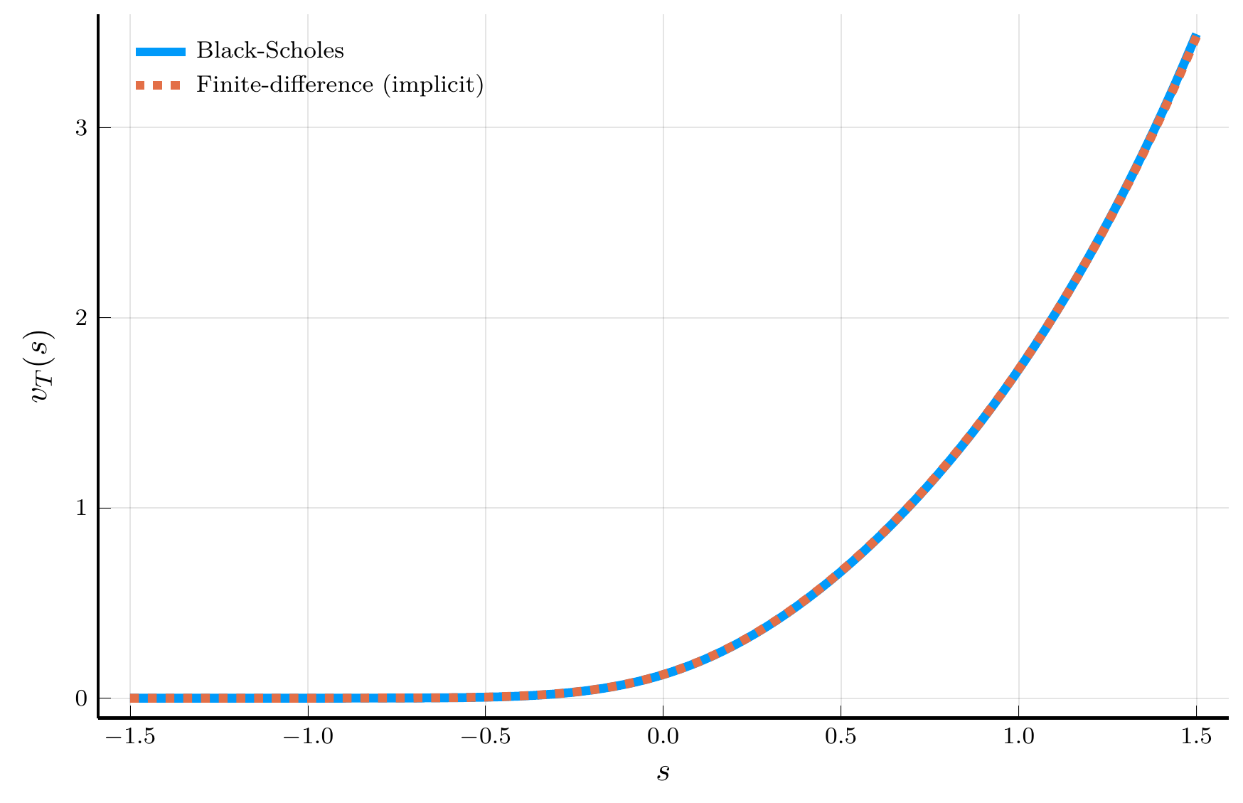
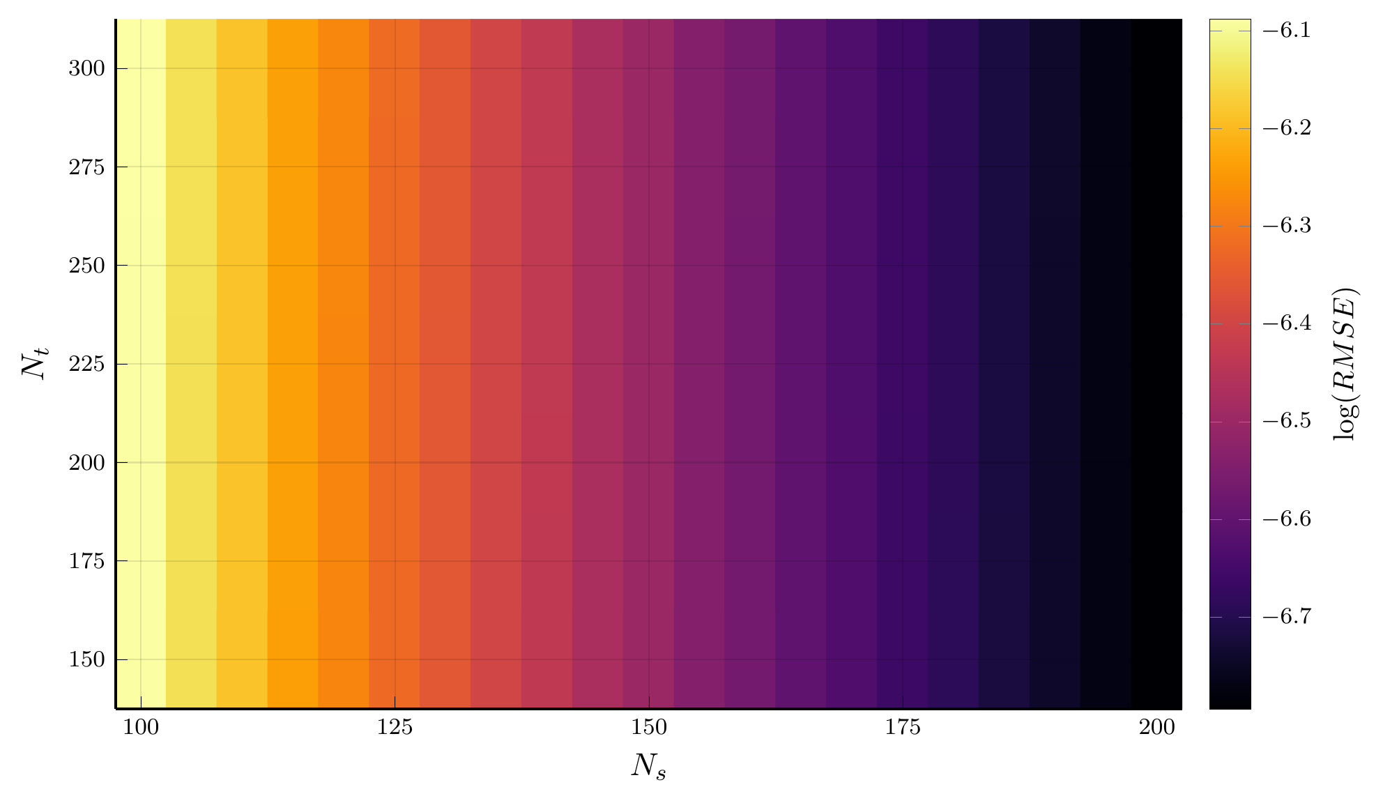
We can plot the solution of the Black–Scholes–Merton PDE using the implicit scheme.

The left panel compares the numerical solution with the exact Black–Scholes–Merton formula.
The right panel shows the error heatmap.
Increasing the number of grid points in the spatial dimension reduces the error.

III. Finite Differences: Income Fluctuations Problem

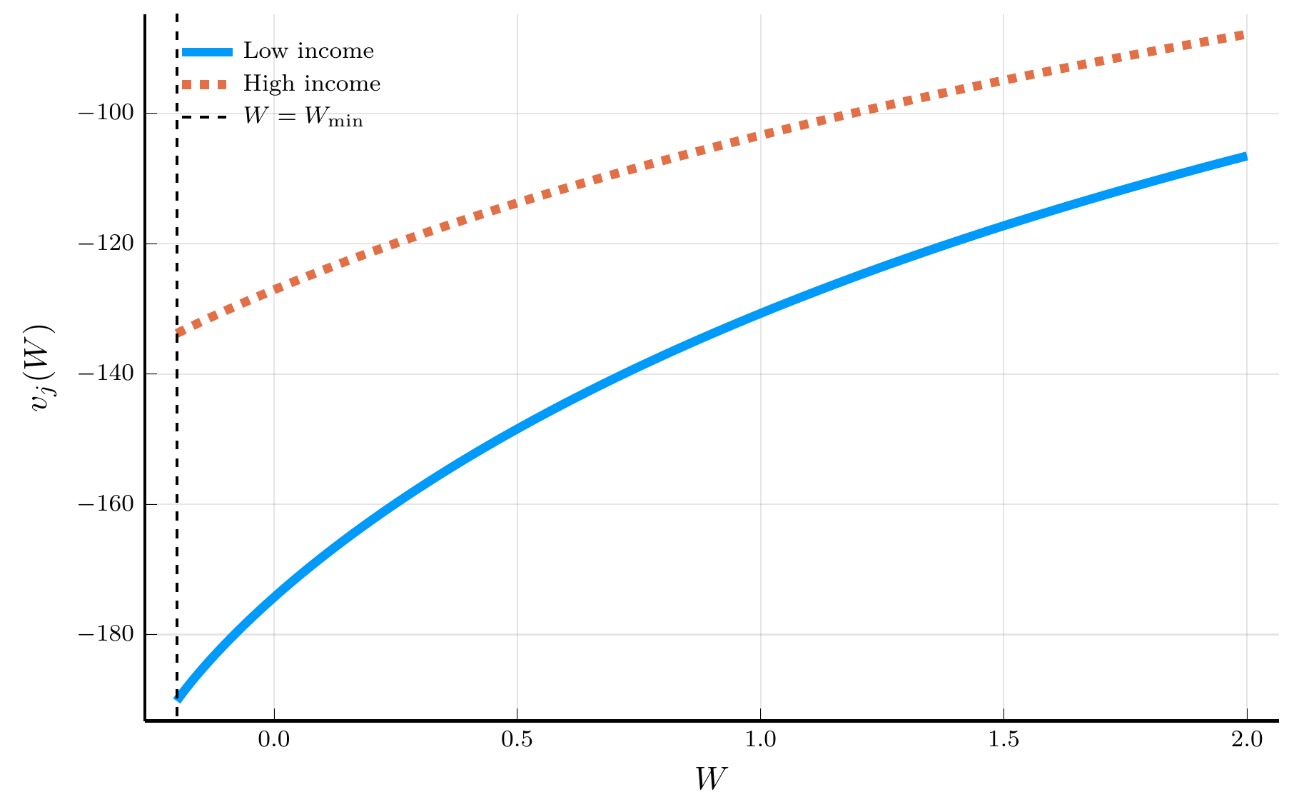
Income Fluctuations Problem

We now solve the income fluctuations problem using a finite-difference scheme.

Relative to the option pricing problem, we must handle (i) the optimal consumption choice and (ii) the borrowing constraint.
Following Achdou et al. (2022), we consider the case without portfolio choice and a two-state income process.

HJB equation: \[ \rho\,V_{j,t}(W) \;=\; u \big(c_{j,t}(W)\big) \;-\; \frac{\partial V_{j,t}}{\partial t}(W) \;+\; \frac{\partial V_{j,t}}{\partial W}(W)\,\big[rW + Y_j - c_{j,t}(W)\big] \;+\; \lambda_j \big[V_{-j,t}(W)-V_{j,t}(W)\big], \] where \(c_{j,t}(W) = u'^{-1}\!\big(V_{j,t}'(W)\big)\) and \(\lambda_j\in\{\lambda_1,\lambda_2\}\) is the outgoing intensity from state \(j\).

Upwinding. Define forward and backward differences for the wealth derivative: \[ v_{i,j,F}^{\,n} \;=\; \frac{v_{i+1,j}^{\,n}-v_{i,j}^{\,n}}{\Delta W}, \qquad v_{i,j,B}^{\,n} \;=\; \frac{v_{i,j}^{\,n}-v_{i-1,j}^{\,n}}{\Delta W}. \] The corresponding wealth drifts are \[ \mu_{i,j,F}^{\,n} \;=\; r W_i + Y_j - u'^{-1}\!\big(v_{i,j,F}^{\,n}\big), \qquad \mu_{i,j,B}^{\,n} \;=\; r W_i + Y_j - u'^{-1}\!\big(v_{i,j,B}^{\,n}\big). \]

The upwinded derivative used in the drift: \[ v_{i,j,W}^{\,n} \;=\; v_{i,j,F}^{\,n}\,\mathbf{1}_{\{\mu_{i,j,F}^{\,n}>0\}} \;+\; v_{i,j,B}^{\,n}\,\mathbf{1}_{\{\mu_{i,j,B}^{\,n}<0\}} \;+\; \overline v_{i,j}\,\mathbf{1}_{\{\mu_{i,j,F}^{\,n}\le 0 \le \mu_{i,j,B}^{\,n}\}}, \] where \(\overline v_{i,j} \equiv u'(rW_i+Y_j)\).

Semi-implicit upwind scheme

Let \([x]^+=\max\{x,0\}\) and \([x]^-=\min\{x,0\}\). The semi-implicit scheme is \[ \rho\,v_{i,j}^{\,n+1} \;=\; u_{i,j}^{\,n} \;-\; \frac{v_{i,j}^{\,n+1}-v_{i,j}^{\,n}}{\Delta t} \;+\; \frac{v_{i+1,j}^{\,n+1}-v_{i,j}^{\,n+1}}{\Delta W}\,[\mu_{i,j,F}^{\,n}]^{+} \;+\; \frac{v_{i,j}^{\,n+1}-v_{i-1,j}^{\,n+1}}{\Delta W}\,[\mu_{i,j,B}^{\,n}]^{-} \;+\; \lambda_j\!\left(v_{i,-j}^{\,n+1}-v_{i,j}^{\,n+1}\right). \] Rearranging, yields the linear system \[ -\ell_{i,j}^{\,n}\,v_{i-1,j}^{\,n+1} \;+\; s_{i,j}^{\,n}\,v_{i,j}^{\,n+1} \;-\; r_{i,j}^{\,n}\,v_{i+1,j}^{\,n+1} \;-\; \lambda_j\,v_{i,-j}^{\,n+1} \;=\; \frac{1}{\Delta t}\,v_{i,j}^{\,n} \;+\; u_{i,j}^{\,n}, \label{eq:semi_implicit_linear} \] with nonnegative coefficients \[ \begin{align} \ell_{i,j}^{\,n} &\equiv -\frac{[\mu_{i,j,B}^{\,n}]^{-}}{\Delta W} \;\ge 0,\\ r_{i,j}^{\,n} &\equiv \;\frac{[\mu_{i,j,F}^{\,n}]^{+}}{\Delta W} \;\ge 0,\\ s_{i,j}^{\,n} &\equiv \frac{1}{\Delta t} \;+\; \ell_{i,j}^{\,n} \;+\; r_{i,j}^{\,n} \;+\; \rho+\lambda_j. \end{align} \]

Boundary conditions

To impose the no-borrowing condition at the lower boundary \(W=\underline W\), and reflection at the upper boundary \(W=\overline W\), set \[ v_{1,j,B}^{\,n} \;=\; u'(rW_1+Y_j), \qquad \qquad v_{N,j,F}^{\,n} \;=\; u'(rW_N+Y_j). \] Hence, by construction, \(\ell_{1,j}^{\,n}=r_{N,j}^{\,n}=0\), so ghost nodes are never used.

Block matrix form

Stack the two income states as \[ \mathbf{v}_j^{\,n} = \big(v_{1,j}^{\,n},\dots,v_{N,j}^{\,n}\big)^\top,\quad \mathbf{v}^{\,n} = \big((\mathbf{v}_1^{\,n})^\top,(\mathbf{v}_2^{\,n})^\top\big)^\top,\quad \mathbf{u}^{\,n} = \big(u(c_{1,1}^{\,n}),\dots,u(c_{N,2}^{\,n})\big)^\top. \] Then \[ \mathbf{A}^{\,n}\,\mathbf{v}^{\,n+1} \;=\; \frac{1}{\Delta t}\,\mathbf{v}^{\,n} + \mathbf{u}^{\,n}, \] with the \(2N\times 2N\) block matrix \[ \mathbf{A}^{\,n} \;=\; \begin{pmatrix} \mathbf{A}_1^{\,n} & -\,\lambda_1\, \mathbf{I}_N \\ -\,\lambda_2\, \mathbf{I}_N & \mathbf{A}_2^{\,n} \end{pmatrix}, \qquad \qquad \mathbf{A}_j^{\,n} = \begin{pmatrix} s_{1,j}^{\,n} & -r_{1,j}^{\,n} & 0 & \ldots & 0 \\ -\ell_{2,j}^{\,n} & s_{2,j}^{\,n} & -r_{2,j}^{\,n} & \ldots & 0 \\ \vdots & \vdots & \vdots & \ddots & \vdots \\ 0 & \ldots & -\ell_{N-1,j}^{\,n} & s_{N-1,j}^{\,n} & -r_{N-1,j}^{\,n} \\ 0 & \ldots & 0 & -\ell_{N,j}^{\,n} & s_{N,j}^{\,n} \end{pmatrix}. \]

Unconditional stability

Off-diagonals of \(\mathbf{A}^{\,n}\) are nonpositive and \((\text{diag}) - \sum_{\text{offdiag}} |\,\cdot\,| = \big[\tfrac{1}{\Delta t} + \rho+\lambda_j + \ell + r\big] - (\ell + r + \lambda_j) = \tfrac{1}{\Delta t} + \rho \,>\, 0\), for each row. Thus \(\mathbf{A}^{\,n}\) is an M-matrix, the scheme is monotone and convergent, and it is unconditionally stable (no CFL restriction on \(\Delta t\)).

Finite Differences as Policy Function Iteration

We have seen that the finite-difference method can be interpreted as an application of the MCA method: \[ \mathbf{v} = \max_{\mathbf{c}} \Big\{ u(\mathbf{c})\,\Delta t + (1-\rho \Delta t)\,\mathbf{P}(\mathbf{c})\,\mathbf{v} \Big\} \;\equiv\; \mathbf{T}\mathbf{v}, \]

One can solve this problem using any method for discrete-time dynamic programming.

The (semi-implicit) finite-difference scheme of Achdou et al. (2022) is closely related to policy function iteration (PFI).
This was pointed out by Phelan and Eslami (2022).

Algorithm: Policy Function Iteration (PFI)

Input: Initial policy \(\mathbf{c}^{(0)}\), tolerance tol

Output: Value \(\mathbf{v}\), policy \(\mathbf{c}\)

Initialize: \(n \gets 0\)

Repeat until \(\|\mathbf{c}^{(n+1)}-\mathbf{c}^{(n)}\| < \text{tol}\):

Policy evaluation:
Solve \([I-(1-\rho\Delta t)P(\mathbf{c}^{(n)})]\mathbf{v}^{(n+1)} = \Delta t\,u(\mathbf{c}^{(n)})\).
Policy improvement:
\(\mathbf{c}^{(n+1)} \gets \arg\max_{\mathbf{c}}\{\Delta t\,u(\mathbf{c})+(1-\rho\Delta t)P(\mathbf{c})\mathbf{v}^{(n)}\}\).
\(n \gets n+1\).

Return: \(\mathbf{v}^{(n)},\,\mathbf{c}^{(n)}\)

Model struct

We start by defining the model parameters and the grid.

@kwdef struct IncomeFluctuationsModel
    ρ::Float64 = 0.05
    r::Float64 = 0.03
    γ::Float64 = 2.0
    Y::Vector{Float64} = [0.1, 0.2]
    λ::Vector{Float64} = [0.02, 0.03]
    Wmin::Float64 = -0.02
    Wmax::Float64 = 2.0
    N::Int64 = 500
    Wgrid::LinRange{Float64} = range(Wmin, Wmax, length = N)
end

Implicit scheme implementation

function fd_implicit(m::IncomeFluctuationsModel; Δt::Float64 = Inf, 
    tol::Float64 = 1e-6, max_iter::Int64 = 100, print_residual::Bool = true)
    (; ρ, r, γ, Y, λ, Wgrid, Wmin, Wmax, N) = m # unpack parameters
    ΔW = Wgrid[2] - Wgrid[1]
    # Initial guess
    v = [1/ρ * (y + r * w)^(1-γ) / (1-γ) for w in Wgrid, y in Y] 
    c, vW, residual = similar(v), similar(v), 0.0 # pre-allocation
    for i = 1:max_iter
        # Compute derivatives
        Dv = (v[2:end,:] - v[1:end-1,:]) / ΔW
        vB = [(@. (r * Wmin + Y)^(-γ))'; Dv] # backward difference
        vF = [Dv; (@. (r * Wmax + Y)^(-γ))'] # forward difference
        v̅  = (r * Wgrid .+ Y').^(-γ) # zero-savings case
        μB = r * Wgrid .+ Y' - vB.^(-1/γ) # backward drift
        μF = r * Wgrid .+ Y' - vF.^(-1/γ) # forward drift
        vW = ifelse.(μF .> 0.0, vF, ifelse.(μB .< 0.0, vB, v̅))
        # Assemble matrix
        c  = vW.^(-1/γ)          # consumption
        u  = c.^(1-γ) / (1-γ)    # utility
        L = -min.(μB, 0) / ΔW    # subdiagonal
        R = max.(μF, 0) / ΔW     # superdiagonal
        S = @. 1/Δt + L + R + ρ + λ' # diagonal
        Aj = [Tridiagonal(-L[2:end,j], S[:,j], -R[1:end-1,j]) 
                for j in eachindex(Y)] # tridiagonal matrices
        A = [sparse(Aj[1]) -λ[1] * I
            -λ[2] * I sparse(Aj[2])] # block matrix
        # Update
        vp = A \ (u + v/Δt)[:]
        residual = sqrt(mean((vp - v[:]).^2)) 
        v = reshape(vp, N, length(Y)) # reshape vector to matrix
        if print_residual println("Iteration $i, residual = $residual") end
        if residual < tol
            break
        end
    end
    s = r * Wgrid .+ Y' - c   # savings
    return (; v, vW, c, s, residual) # return solution
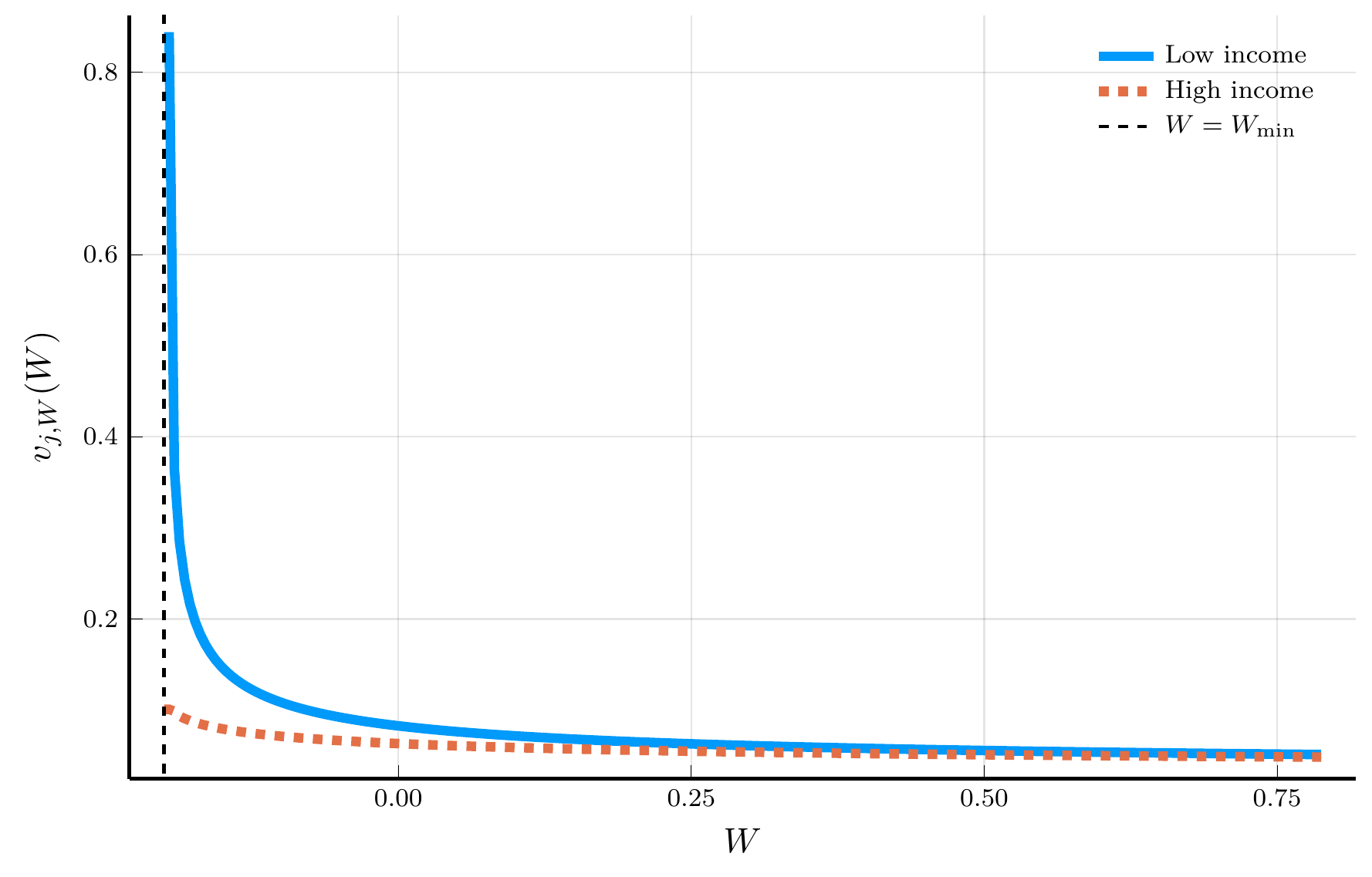
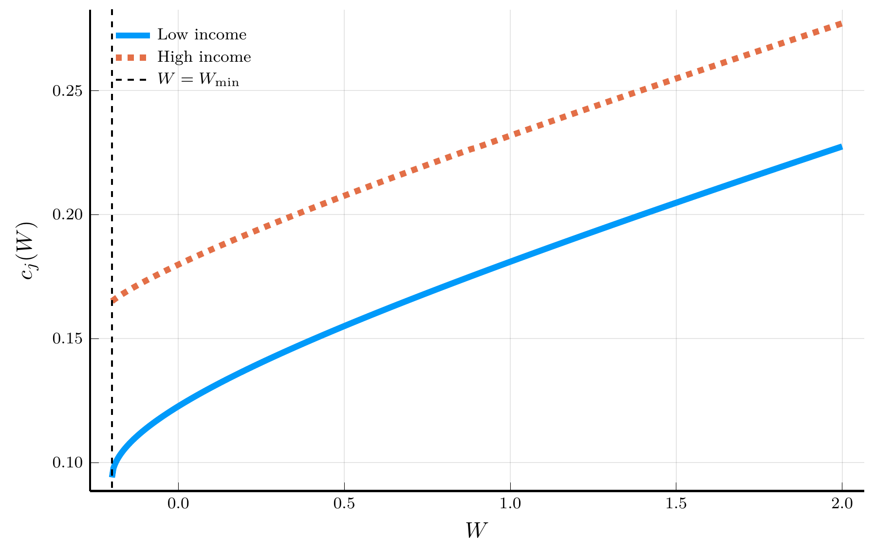
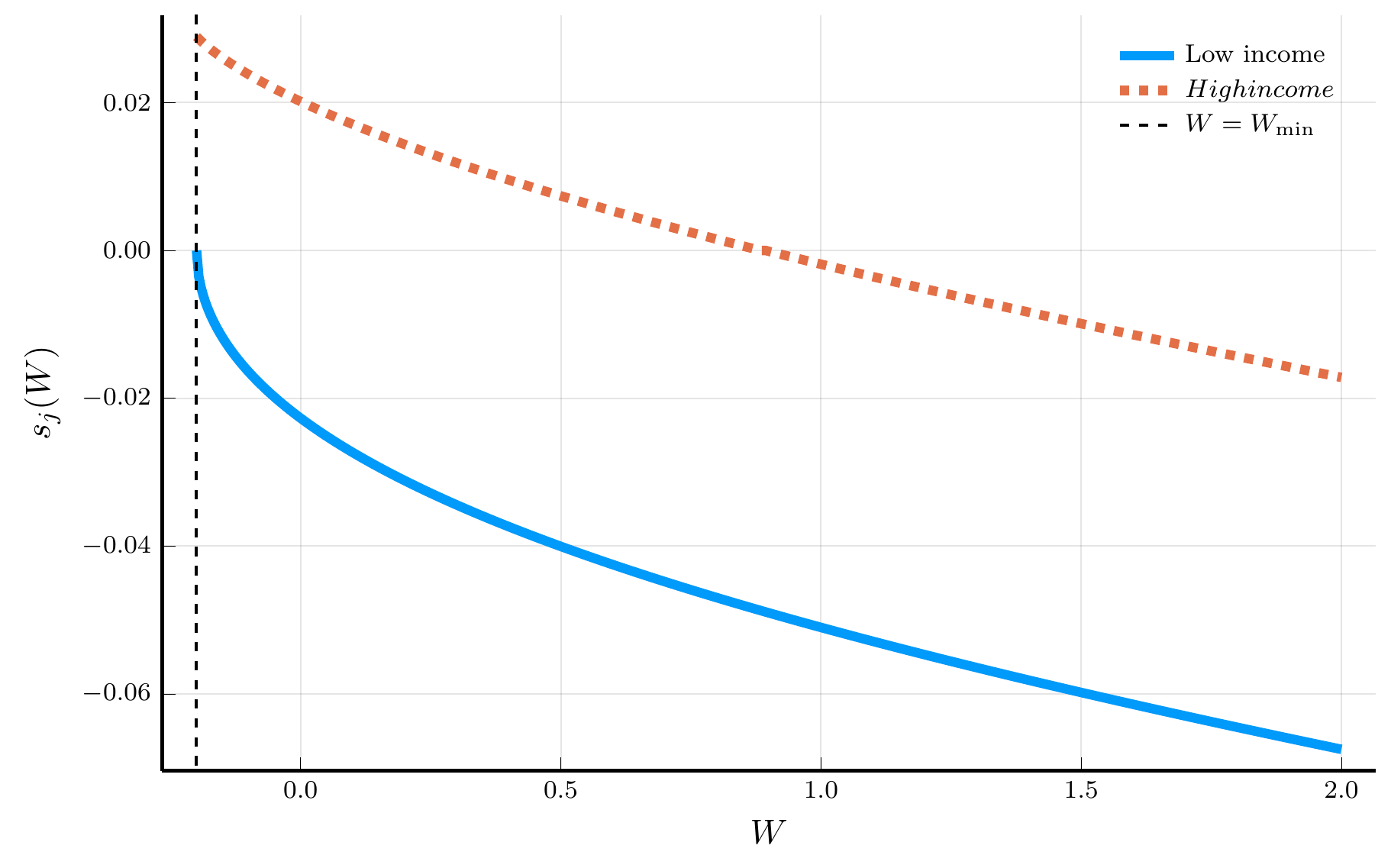
end

The Solution to the Income Fluctuations Problem

IV. Spectral Methods

Finite differences as local polynomial approximations

We have used finite differences to generate a local approximation of derivatives, based on function values at neighboring points.

We will see how to use spectral methods, which instead provide a global approximation of derivatives.
We are interested in computing the derivative of a function \(v(x)\) that we observe at discrete points \(\{x_i\}_{i=1}^N\).

A natural approximation is the forward difference: \[ v'(x_i) = \frac{v_{i+1}-v_i}{\Delta x}+ O(\Delta x). \]

This is equivalent to replacing \(v(x)\) locally by a linear interpolant:

\[ \tilde v(x) = v_i + Dv_i (x-x_i), \qquad Dv_i = \frac{v_{i+1}-v_i}{\Delta x}. \]

Differentiating the interpolant yields \(\tilde v'(x_i)=Dv_i\), i.e., the forward difference.

The central difference formula yields \[ v'(x_i) = \frac{v_{i+1}-v_{i-1}}{2\Delta x} + O(\Delta x^2), \]

This is equivalent to replacing \(v(x)\) by a quadratic interpolant:

\[ \tilde v(x) = \ell_{i-1}(x)v_{i-1} + \ell_i(x)v_i + \ell_{i+1}(x)v_{i+1}, \]

where the basis polynomials are \(\ell_{i-1}(x) = \frac{(x-x_i)(x-x_{i+1})}{2\Delta x^2}\), \(\ell_i(x) = -\frac{(x-x_i+\Delta x)(x-x_i-\Delta x)}{\Delta x^2}\), and \(\ell_{i+1}(x) = \frac{(x-x_i+\Delta x)(x-x_i)}{2\Delta x^2}\).

Differentiating and evaluating at \(x_i\) yields the central difference formulas: \[ \tilde v'(x_i) = \frac{v_{i+1}-v_{i-1}}{2\Delta x}, \qquad \tilde v''(x_i) = \frac{v_{i+1}-2v_i+v_{i-1}}{\Delta x^2}, \]

Higher-order finite differences

We can obtain higher-order finite-difference formulas by fitting higher-degree local polynomials and differentiating them.

For example, a quartic interpolant yields a fourth-order approximation to \(v'(x_i)\).
We can compute such higher-order approximations in Julia using the Polynomials.jl package.

"""
    finite_difference(f, x0, accuracy; scheme=:forward, Δx=0.01)

Approximate f'(x0) by differentiating a local interpolating 
polynomial built on a stencil that achieves the requested accuracy.
"""
function finite_difference(f::Function, x0::Float64, accuracy::Int;
                    scheme::Symbol = :forward, Δx::Float64 = 0.01)
    @assert accuracy > 0 "accuracy order must be positive"
    steps = zeros(Int, accuracy+1)
    if iseven(accuracy)
        m = accuracy ÷ 2
        steps = collect(-m:m)
    else
        q = accuracy
        steps = scheme === :forward ? collect(0:q) : collect(-q:0)
    end
    x_points = x0 .+ Δx .* steps
    p    = Polynomials.fit(x_points, f.(x_points), length(x_points) - 1)
    return Polynomials.derivative(p)(x0)
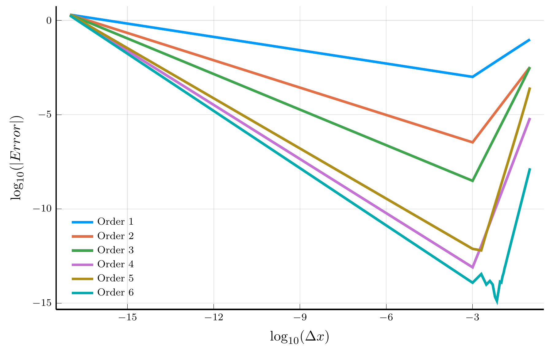
end

Truncation vs. Roundoff Error

One would expect that the error of the finite-difference approximation decreases as the grid is refined (\(\Delta x \to 0\)).

However, eventually the error increases again as \(\Delta x\) becomes very small.
This is due to the interplay of truncation error and roundoff error.

From local to global polynomials

Suppose we approximate a smooth function \(v(x)\) on \([-1,1]\) by a single polynomial of degree \(N\): \[\begin{equation} v(x) \approx \tilde v_N(x) = \sum_{k=0}^{N} a_k x^k, \end{equation}\] where the coefficients \(a_k\) are chosen so that \(\tilde v_N(x_i) = v(x_i)\) at a set of interpolation nodes \(\{x_i\}_{i=0}^N\).

Change of domain

When approximating a function \(v(x)\) on a bounded domain \([a,b]\), we can always map it to the interval \([-1,1]\) via \[ v(x) \equiv V\!\left(\tfrac{(b-a)x + (a+b)}{2}\right), \qquad x \in [-1,1]. \] For a discussion of approximations on unbounded domains, see Chapter 17 of Boyd (2001).

Finite vs. spectral accuracy

Higher-order finite differences improve accuracy algebraically, with error \(O(\Delta x^p)\) for a \(p\)-th order scheme.

In contrast, spectral methods achieve exponential (or spectral) convergence for smooth functions, as we will see next.

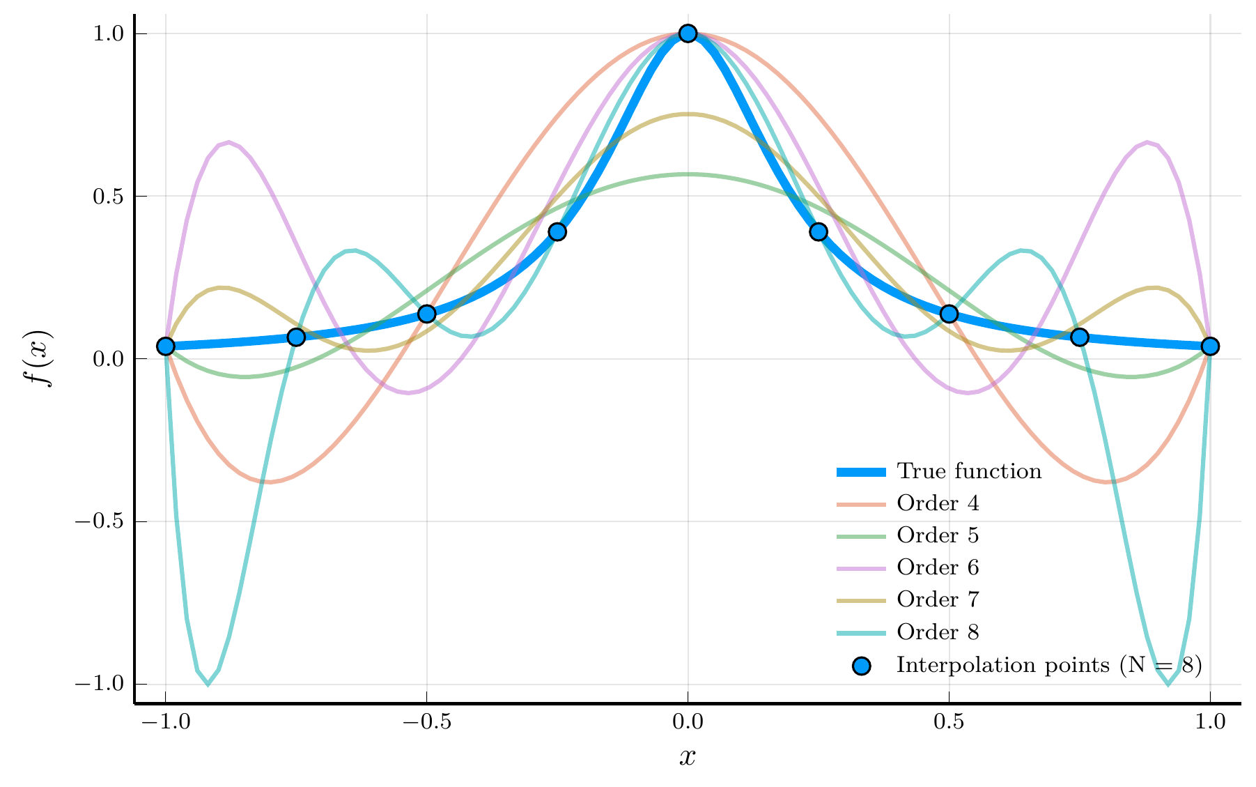
The Runge phenomenon

This global approach uses information from the entire domain to approximate derivatives or other operators.

However, if the interpolation nodes \(x_i\) are equally spaced, the interpolant may oscillate violently near the boundaries as \(N\) increases
A pathology known as the Runge phenomenon: consider the function \(v(x) = \frac{1}{1 + 25x^2}\), for \(x \in [-1,1]\).

The interpolation error theorem

The interpolation error theorem 🌐 provides a useful decomposition of the interpolation error.

Let \(v(x)\) have at least \(N+1\) derivatives on \([-1,1]\) and let \(\tilde v_N(x)\) be the degree-\(N\) interpolant of \(v(x)\) at nodes \(\{x_i\}_{i=0}^N\).
Then, the interpolation error is given by \[ v(x) - \tilde v_N(x) = \color{#0072b2}{\frac{v^{(N+1)}(\xi)}{(N+1)!}}\,\color{#009e73}{\mathcal{P}_{N+1}(x)}, \qquad \mathcal{P}_{N+1}(x) = \prod_{i=0}^{N}(x - x_i), \] for some \(\xi \in [-1,1]\).

The error therefore depends on two components:

The \((N+1)\)-st derivative \(v^{(N+1)}(\xi)\), which depends only on the smoothness of \(v\); and
The node polynomial \(\mathcal{P}_{N+1}(x)\), which depends solely on the choice of interpolation nodes.

We cannot control the smoothness of \(v\), but we can control the second term.

Worst-case interpolation error

The worst-case (uniform) interpolation error is bounded by \[ |v(x) - \tilde v_N(x)| \le \frac{1}{(N+1)!}\, \max_{x \in [-1,1]} |v^{(N+1)}(x)|\, \|\mathcal{P}_{N+1} \|_\infty, \qquad \|\mathcal{P}_{N+1} \|_\infty \equiv \max_{x \in [-1,1]} |\mathcal{P}_{N+1}(x)|. \]

Chebyshev polynomials and the minimax property

Our goal is clear: choose interpolation nodes \(\{x_i\}\) that minimize \(\|\mathcal{P}_{N+1}\|_\infty\).

This leads directly to the Chebyshev minimal amplitude theorem.

Chebyshev minimal amplitude theorem

Define the Chebyshev nodes🌐 as \[ \hat{x}_i = \cos\!\left(\frac{(2i+1)\pi}{2(N+1)}\right), \qquad i = 0,\ldots,N. \] The polynomial \(\mathcal{P}_{N+1}(x) = \prod_{i=0}^{N} (x - x_i)\) attains its smallest maximum amplitude on \([-1,1]\) when the \(x_i\) are the Chebyshev nodes: \[ \|\mathcal{P}_{N+1}\|_\infty = \max_{x \in [-1,1]} |\mathcal{P}_{N+1}(x)| \geq \max_{x \in [-1,1]} \left|\prod_{i=0}^{N} (x - \hat{x}_i)\right|. \]

Chebyshev nodes are the roots of the Chebyshev polynomial 🌐, \[ T_{N+1}(x) = \cos\!\big((N+1)\arccos x\big), \] which oscillates between \(-1\) and \(1\) exactly \(N{+}2\) times on \([-1,1]\).

Chebyshev polynomials enjoy an orthogonality relation: \[ \int_{-1}^1 T_m(x)\,T_n(x)\,w(x)\,dx = 0, \qquad m \ne n, \qquad w(x)=1/\sqrt{1-x^2}. \]

From interpolation to differentiation

Let \(\tilde v_N(x) = \sum_{k=0}^N a_k T_k(x)\) be the degree-\(N\) Chebyshev interpolant of \(v(x)\):

Given the interpolant, it is straightforward to compute its derivatives.
One can use recursion for Chebyshev polynomials of the second kind or the formulas in the lecture notes.

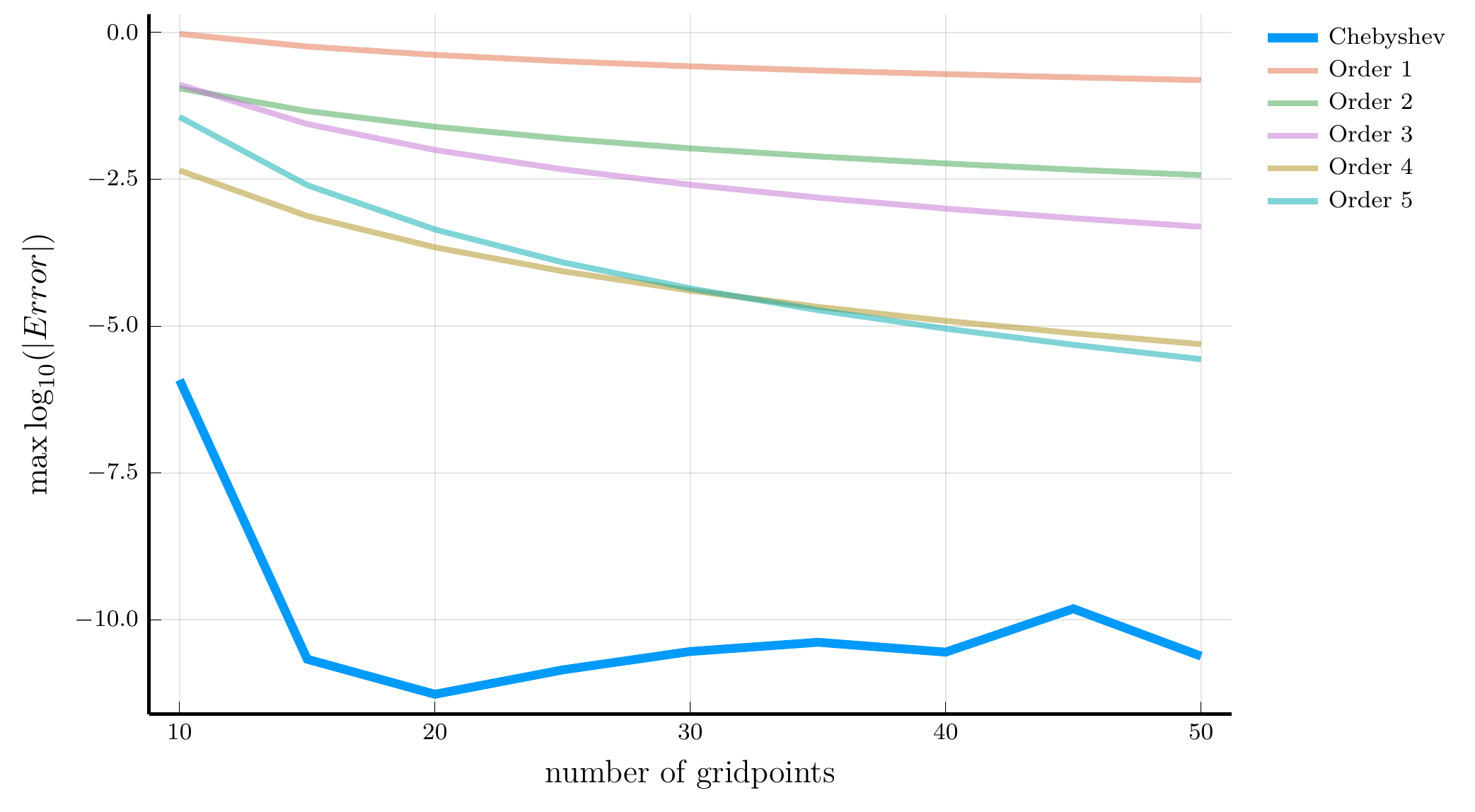
Consider the smooth function \(v(x) = e^{x^2} + 2\sin(x)\):

The figure shows the approximation error for the derivative
We compare finite differences and Chebyshev differentiation

Chebyshev differentiation reaches machine precision accuracy

With a modest number of nodes (around \(N=20\))
Even with \(N = 10\), it is orders of magnitude more accurate than FD

Derivatives of Chebyshev polynomials

Because the Chebyshev interpolation error decays exponentially for smooth functions, the same holds for the derivative approximation: \[ \|\tilde v_N'(x) - v'(x)\|_\infty = O(e^{-\alpha N}), \qquad \text{for some } \alpha >0. \]

The Two-trees Model

We can use Chebyshev polynomials to solve PDEs like the HJB equation

To illustrate the method, we consider the two-trees model of Cochrane, Longstaff, and Santa-Clara (2008)
The model is a two-tree economy with dividends following a geometric Brownian motion: \[ \frac{d D_{i,t}}{D_{i,t}} = \mu dt + \sigma dB_{i,t}, \qquad i = 1,2. \]

Aggregate consumption equals the sum of dividends from the two trees: \(C_t = D_{1,t} + D_{2,t}\).

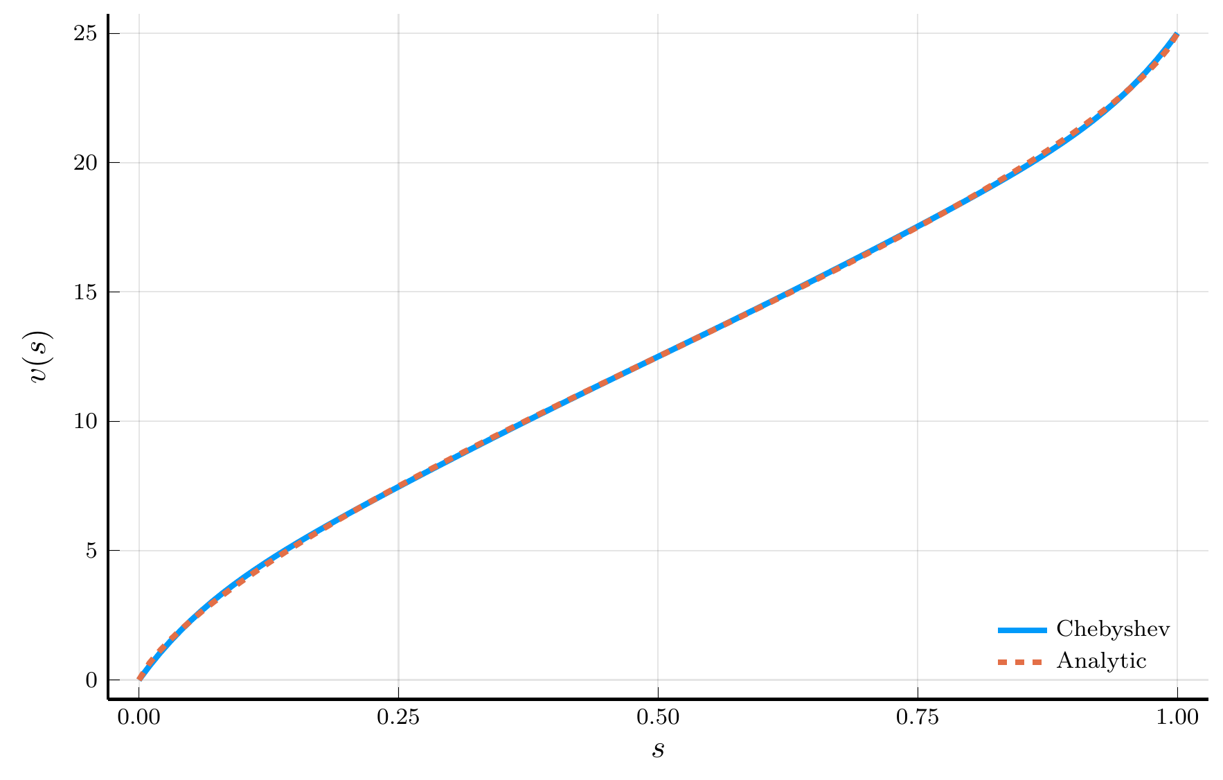
Assuming the representative household has log utility, the price of the first tree is given by: \[ P_{t} = \mathbb{E}_t \left[ \int_{0}^{\infty} e^{-\rho s} \frac{C_t}{C_{t+s}} D_{1,t+s} ds \right] \Rightarrow v_{t} = \mathbb{E}_t \left[ \int_{0}^{\infty} e^{-\rho s} s_{t+s} ds \right], \qquad v_t \equiv \frac{P_t}{C_t}, \qquad s_t \equiv \frac{D_{1,t}}{C_{t}}. \]

The HJB equation

The price-consumption ratio \(v_t\) satisfies the HJB equation: \[ \rho v = s - v_s \,2\sigma^2 s(1-s)\!\left(s-\tfrac12\right) + \frac{1}{2} v_{ss}\,\big(2\sigma^2 s^2(1-s)^2\big), \] with boundary conditions \(v(0) = 0\) and \(v(1) = 1/\rho\), using \(d s_t = - 2 \sigma^2 s_t(1-s_t)(s_t -1/2) dt + \sigma s_t(1-s_t)(dB_{1,t}- dB_{2,t})\).

Solving the HJB equation with Chebyshev collocation

To solve the HJB equation with Chebyshev collocation, we start with a series expansion of \(v(s)\): \[ v(s) = \sum_{n=0}^{\infty} a_n \tilde{T}_n(s) \approx \sum_{n=0}^{N} a_n \tilde{T}_n(s), \qquad \qquad \tilde{T}_n(s) = T_n(2s-1). \]

Change of domain

The mapping \(s \mapsto x=2s-1\) rescales the domain from \([0,1]\) to \([-1,1]\), allowing the use of standard Chebyshev polynomials. Derivatives with respect to \(s\) follow from the chain rule, yielding \(\tilde T_n'(s)=2T_n'(2s-1)\) and \(\tilde T_n''(s)=4T_n''(2s-1)\).

Plugging the expansion into the HJB equation and evaluating at the grid points, we obtain the linear system: \[ \mathbf{L} \mathbf{a} = \mathbf{b}, \] where \(\mathbf{L}\) is a \((N+1) \times (N+1)\) matrix and \(\mathbf{b}\) is a \((N+1)\) vector.

Interior points. For \(i =2,\ldots,N\) and \(j = 1,\ldots,N+1\), we have: \[ \mathbf{L}_{i,j} \;=\; \rho\,\tilde T_{j-1}(s_i) \;+\; 2\sigma^2 s_i(1-s_i)\!\left(s_i-\tfrac12\right)\,\tilde T_{j-1}'(s_i) \;-\; \sigma^2 s_i^2(1-s_i)^2\,\tilde T_{j-1}''(s_i), \qquad \qquad b_i = s_i. \]

Boundary conditions

The first and last rows accommodate the boundary conditions: \[ \begin{align} \mathbf{L}_{1,j} &= \tilde{T}_{j-1}(0), \qquad \mathbf{L}_{N+1,j} = \tilde{T}_{j-1}(1), \qquad \qquad b_1 = 0, \qquad b_{N+1} = 1/\rho. \end{align} \]

Julia Implementation

We start by defining the model structure for the two-trees model:

@kwdef struct TwoTrees
    ρ::Float64 = 0.04
    σ::Float64 = sqrt(0.04)
    μ::Float64 = 0.02
    N::Int = 7
end

To construct the matrix \(\mathbf{L}\), we need to evaluate the Chebyshev polynomials and their derivatives at the grid points:

We use the implementation of Chebyshev polynomials and their derivatives from the Polynomials.jl package.

function chebyshev_derivatives(n::Int, z::Real; 
        zmin::Real = -1.0, zmax::Real = 1.0)
    a, b = 2 / (zmax - zmin), -(zmin + zmax) / (zmax - zmin)
    x = a * z + b # Map to [-1,1]
    p = ChebyshevT([zeros(n);1.0]) # Degree n Chebyshev polynomial
    d1p = derivative(p) # First derivative
    d2p = derivative(d1p) # Second derivative
    return p(x), d1p(x) * a, d2p(x) * a^2
end

The Chebyshev solver

The function chebyshev_solver solves for the coefficients \(a_n\) of the Chebyshev expansion of the price-consumption ratio \(v(s)\):

The function returns a NamedTuple with the function \(v(s)\) and the grid \(s_i\).
Notice that the function \(v(s)\) can be evaluated at any point in the interval \([z_{\min},z_{\max}]\), not just the grid points.

function chebyshev_solver(m::TwoTrees)
    (; ρ, σ, N) = m
    # Chebyshev grid and mapping to [0,1]
    x = reverse(cos.(pi .* (0:N) ./ N))
    s = (x .+ 1) ./ 2
    # Assemble the linear operator
    L, b = zeros(N+1, N+1), copy(s)
    for i in 1:N+1, j in 1:N+1
        T̃, dT, d2T = chebyshev_derivatives(j-1, s[i]; zmin = 0)
        if i == 1 || i == N+1
            L[i,j] = T̃ # Boundary points
        else
            μs = -2 * σ^2 * s[i] * (1 - s[i]) * (s[i] - 1/2)
            σs = sqrt(2) * σ * s[i] * (1 - s[i])
            L[i,j] = ρ * T̃ - dT * μs - d2T * σs^2 / 2
        end
    end
    b[end] = 1/ρ # Boundary condition at s = 1
    a = L \ b  # Solve for the coefficients
    return (; v = z -> ChebyshevT(a)(2 * z - 1), s = s) 
end

The Solution of the Two-trees Model

The Challenge of High-Dimensional Problems Redux

Finite Difference Methods in High-Dimensional Problems

We have seen how to use finite-difference and Chebyshev collocation methods to continuous time models.

These techniques are very effective in one or two dimensions.
However, they suffer from the same three curses of dimensionality as in the discrete-time setting.

Finite-difference schemes in higher dimensions.

Because finite-difference schemes represent the state space on a grid, they inherit the first curse of dimensionality.
The number of grid points grows exponentially with the number of state variables

A second difficulty is maintaining the monotonicity of the scheme.

It is straightforward to guarantee monotonicity in one dimension
In higher dimensions, however, cross-derivative terms create complications.
Consider an HJB equation with two state variables \(\mathbf{s} = (s_1, s_2)\):

\[ \rho v = u(\mathbf{s}) + v_{s_1}\,\mu_{s_1}(\mathbf{s}) + v_{s_2}\,\mu_{s_2}(\mathbf{s}) + \tfrac{1}{2}v_{s_1s_1}\,\sigma_{s_1}^2(\mathbf{s}) + \tfrac{1}{2}v_{s_2s_2}\,\sigma_{s_2}^2(\mathbf{s}) + v_{s_1s_2}\,\sigma_{s_1s_2}(\mathbf{s}). \]

A central-difference approximation for the mixed derivative, \[ v_{s_1s_2} \approx \frac{v_{i+1,j+1} - v_{i-1,j-1} - v_{i+1,j-1} + v_{i-1,j+1}} {4 \Delta s_1 \Delta s_2}, \] produces nonnegative off-diagonal elements in the discretization matrix, violating the M-matrix conditions required for stability.

Chebyshev Collocation in High-Dimensional Problems

Chebyshev collocation methods share the same first curse.

In one dimension, they achieve exponential accuracy with relatively few nodes.
In \(d\) dimensions, however, the tensor product of one-dimensional bases yields \((N+1)^d\) nodes.

Several strategies mitigate this explosion.

Judd et al. (2014) propose Smolyak sparse grids and anisotropic tensor-product bases
This dramatically reduces the number of collocation points.
However, these approaches face steep scaling once \(d\) exceeds five to ten dimensions.

The need for new methods

Both finite-difference and collocation methods ultimately confront the same exponential barriers as their discrete-time counterparts.

In the next modules, we explore modern machine-learning-based approaches that circumvent these limitations.

References

Achdou, Yves, Jiequn Han, Jean-Michel Lasry, Pierre-Louis Lions, and Benjamin Moll. 2022. “Income and Wealth Distribution in Macroeconomics: A Continuous-Time Approach.” The Review of Economic Studies 89 (1): 45–86.

Barles, Guy, and Panagiotis E. Souganidis. 1991. “Convergence of Approximation Schemes for Fully Nonlinear Second Order Equations.” Asymptotic Analysis 4: 271–83.

Boyd, John P. 2001. Chebyshev and Fourier Spectral Methods. Mineola, NY: Dover Publications.

Cochrane, John H., Francis A. Longstaff, and Pedro Santa-Clara. 2008. “Two Trees.” The Review of Financial Studies 21 (1): 347–85. https://doi.org/10.1093/rfs/hhm059.

Judd, Kenneth L., Lilia Maliar, Serguei Maliar, and Rafael Valero. 2014. “Smolyak Method for Solving Dynamic Economic Models: Lagrange Interpolation, Anisotropic Grid and Adaptive Domain.” Journal of Economic Dynamics and Control 44: 92–123. https://doi.org/10.1016/j.jedc.2014.03.005.

Kushner, Harold J., and Paul G. Dupuis. 2001. Numerical Methods for Stochastic Control Problems in Continuous Time. 2nd ed. Applications of Mathematics 24. New York: Springer.

Phelan, Thomas, and Keyvan Eslami. 2022. “Applications of Markov Chain Approximation Methods to Optimal Control Problems in Economics.” Journal of Economic Dynamics and Control 143: 104437. https://doi.org/10.1016/j.jedc.2022.104437.