Machine Learning for Computational Economics

Module 05: The Deep Policy Iteration Method
EDHEC Business School

Dejanir Silva

Purdue University

January 2026

Introduction

In this module, we use machine-learning tools to solve high-dimensional problems in continuous time.

• We introduce the Deep Policy Iteration (DPI) method, proposed by Duarte, Duarte, and Silva (2024).
• It combines stochastic optimization, automatic differentiation, and neural-network function approximation.

We proceed in two steps.

1. We show how to overcome the three curses of dimensionality.
2. We describe a range of applications of the DPI method in asset pricing, corporate finance, and portfolio choice.

The module is organized as follows:

1. The Hyper-Dual Approach to Itô’s lemma
2. The DPI Method
3. Applications

I. Dealing with the Three Curses

The Dynamic Programming Problem

Consider a continuous-time optimal control problem in which an infinitely lived agent faces a Markovian decision process (MDP).

• The system’s state is represented by a vector \(\mathbf{s}_t \in \mathbb{R}^n\)
• The control is a vector \(\mathbf{c}_t \in \Gamma(\mathbf{s}_t) \subset \mathbb{R}^p\).

The agent’s objective is to maximize the expected discounted value of the reward function \(u(\mathbf{c}_t)\): \[ V(\mathbf{s}) = \max_{\{\mathbf{c}_t\}_{t=0}^\infty} \mathbb{E}\left[ \left. \int_{0}^\infty e^{-\rho t} u(\mathbf{c}_t) dt \right| \mathbf{s}_0 = \mathbf{s} \right], \] subject to the stochastic law of motion \[ d\mathbf{s}_t = \mathbf{f}(\mathbf{s}_t, \mathbf{c}_t) dt + \mathbf{g}(\mathbf{s}_t, \mathbf{c}_t) d\mathbf{B}_t. \] where \(\mathbf{B}_t\) is an \(m \times 1\) vector of Brownian motions, \(\mathbf{f}(\mathbf{s}_t, \mathbf{c}_t) \in \mathbb{R}^n\) is the drift, and \(\mathbf{g}(\mathbf{s}_t, \mathbf{c}_t) \in \mathbb{R}^{n\times m}\) is the diffusion matrix.

The HJB Equation.

The value function \(V(\mathbf{s})\) satisfies the Hamilton–Jacobi–Bellman (HJB) equation: \[ 0 = \max_{\mathbf{c}\in\Gamma(\mathbf{s})} u(\mathbf{c}) - \rho V(\mathbf{s}) + \nabla_{\mathbf{s}} V(\mathbf{s}) \cdot \mathbf{f}(\mathbf{s},\mathbf{c}) + \tfrac{1}{2} \operatorname{Tr}(\mathbf{g}(\mathbf{s},\mathbf{c}) \mathbf{H}_{\mathbf{s}} V(\mathbf{s}) \mathbf{g}(\mathbf{s},\mathbf{c})), \] where \(\nabla_{\mathbf{s}} V(\mathbf{s})\) and \(\mathbf{H}_{\mathbf{s}} V(\mathbf{s})\) denote, respectively, the gradient and Hessian of the value function.

Dealing with the Three Curses

As discussed in Module 1, dynamic programming methods face three intertwined computational obstacles:

1^st curse

Representing \(V(\mathbf{s})\)

2^nd curse

Solving for \(\mathbf{c}\) given \(V(\mathbf{s})\)

3^rd curse

Computing \(\mathbb{E}[V(\mathbf{s}')]\)

In this module, we present an algorithm that addresses each of these curses using modern machine-learning tools:

1. Neural networks provide compact representations of value and policy functions, circumventing the curse of representation;
2. Stochastic optimization replace costly root-finding procedures, alleviating the curse of optimization;
3. Automatic differentiation enables efficient computation of drift terms needed for the HJB, mitigating the curse of expectation;

II. Overcoming the Curse of Expectation

From integration to differentiation

In discrete time, the Bellman equation involves the expectation of the continuation value: \[ \mathbb{E}[V(\mathbf{s}')] = \int \!\!\cdots\!\! \int V(\mathbf{s} + \mathbf{f}(\mathbf{s},\mathbf{c}) \Delta t + \mathbf{g}(\mathbf{s},\mathbf{c}) \sqrt{\Delta t} \mathbf{Z}) \phi(\mathbf{Z}) d\mathbf{Z}_1 \cdots d\mathbf{Z}_m, \] where \(\phi(\mathbf{Z})\) is the joint density of the shocks.

In continuous time, the expected change in the value function can be written as \[ \mathbb{E}[d V(\mathbf{s})] = \nabla_{\mathbf{s}} V(\mathbf{s}) \cdot \mathbf{f}(\mathbf{s},\mathbf{c}) + \tfrac{1}{2} \operatorname{Tr}(\mathbf{g}(\mathbf{s},\mathbf{c}) \mathbf{H}_{\mathbf{s}} V(\mathbf{s}) \mathbf{g}(\mathbf{s},\mathbf{c})), \]

Hence, instead of computing high-dimensional integrals, we only need to compute derivatives of the value function.

Computational challenge.

One could use finite differences to compute these derivatives

• But storing the solution on a grid becomes infeasible in higher dimensions.

Suppose \(n=10\) and we use a grid of 100 points for each state variable.

• Then, just to store the grid in memory, we would need \(10^{17}\) terabytes of RAM.

Comparing the Computational Costs

To illustrate the computational challenge, we study a simple example.

Consider the following function: \[ V(\mathbf{s}) = \sum_{i=1}^n s_i^2, \] where \(\mathbf{s} = (s_1, \ldots, s_n)\) is a vector of state variables.

A high-dimensional problem with \(n=100\) state variables

• We evaluate the drift at the point \(\mathbf{s} = \mathbf{1}_{n\times1}\).
• We focus on the case of a single shock (\(m=1\)).

We consider initially the following methods to compute the drift \(\mathbb{E}[d V(\mathbf{s})]\):

1. Finite differences
2. Naive autodiff

Comparing the Computational Costs.

Method	FLOPs	Memory	Error
1. Finite differences	9,190,800	112,442,048	1.58%
2. Naive autodiff	2,100,501	25,673,640	0.00%

Even the naive autodiff method is computationally costly and memory intensive.

• The naive method computes the Hessian by nested calls to the Jacobian function

Overcoming the Curse of Expectation

One of the key insights from Module 4 is that the Jacobian–vector product (JVP) can be efficiently computed.

• Much less expensive than forming the full Jacobian.

In the absence of shocks, computing the drift of \(V(\mathbf{s})\) amounts to evaluating a JVP:

\[ \mathbb{E}[d V(\mathbf{s})] = \nabla_{\mathbf{s}} V(\mathbf{s})^\top \mathbf{f}(\mathbf{s},\mathbf{c}) dt, \] which can be efficiently computed using forward-mode AD.

In the presence of shocks, the drift also depends on quadratic forms involving the Hessian of \(V(\mathbf{s})\).

• In this case, a JVP is no longer sufficient.

The Hyper-dual approach to Itô’s lemma extends the idea of dual numbers to compute the drift of \(V(\mathbf{s})\).

• Regular dual numbers only store the function value and its derivative.
• Hyper-dual numbers store the function value, its drift, and its diffusion matrix.

The Hyper-Dual Approach to Itô’s lemma

The next result formalizes the hyper-dual approach to Itô’s lemma.

• It reduces the problem of computing the drift of \(V(\mathbf{s})\) to evaluating the second derivative of a univariate auxiliary function.

Hyper-dual Itô’s lemma

For a given \(\mathbf{s}\), define the auxiliary functions \(F_i:\mathbb{R}\rightarrow\mathbb{R}\) as \[ F_i(\epsilon;\mathbf{s}) = V\!\left(\mathbf{s} + \tfrac{\mathbf{g}_i(\mathbf{s})}{\sqrt{2}}\,\epsilon + \tfrac{\mathbf{f}(\mathbf{s})}{2m}\,\epsilon^2 \right), \] where \(\mathbf{f}(\mathbf{s})\) is the drift of \(\mathbf{s}\) and \(\mathbf{g}_i(\mathbf{s})\) is the \(i\)-th column of the diffusion matrix \(\mathbf{g}(\mathbf{s})\).

Then:

Diffusion: The \(1\times m\) diffusion matrix of \(V(\mathbf{s})\) is \[ \nabla V(\mathbf{s})^{\top}\mathbf{g}(\mathbf{s}) = \sqrt{2}\,[F_1'(0;\mathbf{s}), F_2'(0;\mathbf{s}), \ldots, F_m'(0;\mathbf{s})]. \]

Drift: The drift of \(V(\mathbf{s})\) is \[ \mathcal{D}V(\mathbf{s}) = F''(0;\mathbf{s}), \qquad \text{where} \quad F(\epsilon;\mathbf{s}) = \sum_{i=1}^m F_i(\epsilon;\mathbf{s}) \]

An implication of the hyper-dual approach is that the computational complexity is \[ \mathcal{O}(m \times \text{cost}(V(\mathbf{s}))), \] which is independent of the number of state variables.

Julia Implementation

It is straightforward to implement the hyper-dual approach to Itô’s lemma in Julia.

using ForwardDiff, LinearAlgebra
V(s) = sum(s.^2) # example function
n, m  = 100, 1 # number of state variables and shocks
s0, f, g = ones(n), ones(n), ones(n,m) # example values

# Analytical drift
∇f, H = 2*s0, Matrix(2.0*I, n,n) # gradient and Hessian
drift_analytical = ∇f'*f + 0.5*tr(g'*H*g) # analytical drift

# Hyper-dual approach
F(ϵ) = sum([V(s0 + g[:,i]*ϵ/sqrt(2) + f/(2m)*ϵ^2) for i = 1:m])
drift_hyperdual = ForwardDiff.derivative(ϵ -> ForwardDiff.derivative(F, ϵ), 0.0) # scalar 2nd derivative

To verify correctness, we can compare the analytical and hyper-dual drifts:

# Compare
drift_analytical, drift_hyperdual

(300.0, 300.0)

Computational Cost

This figure shows how the cost of computing the drift of a function \(V\) scales with the number of state variables and Brownian shocks.

• The cost is independent of the number of state variables.
• It increases linearly — instead of exponentially — with the number of Brownian shocks.

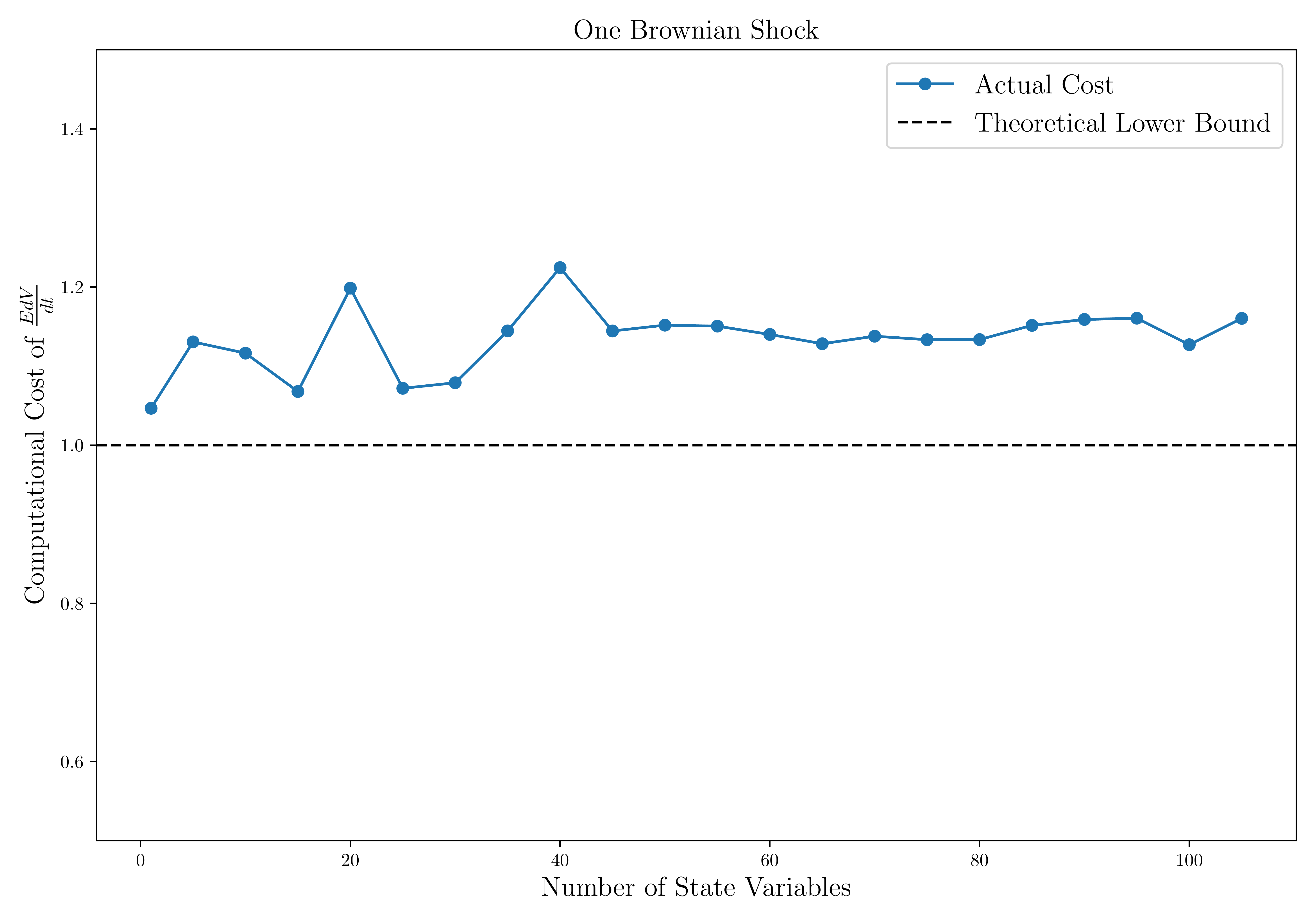
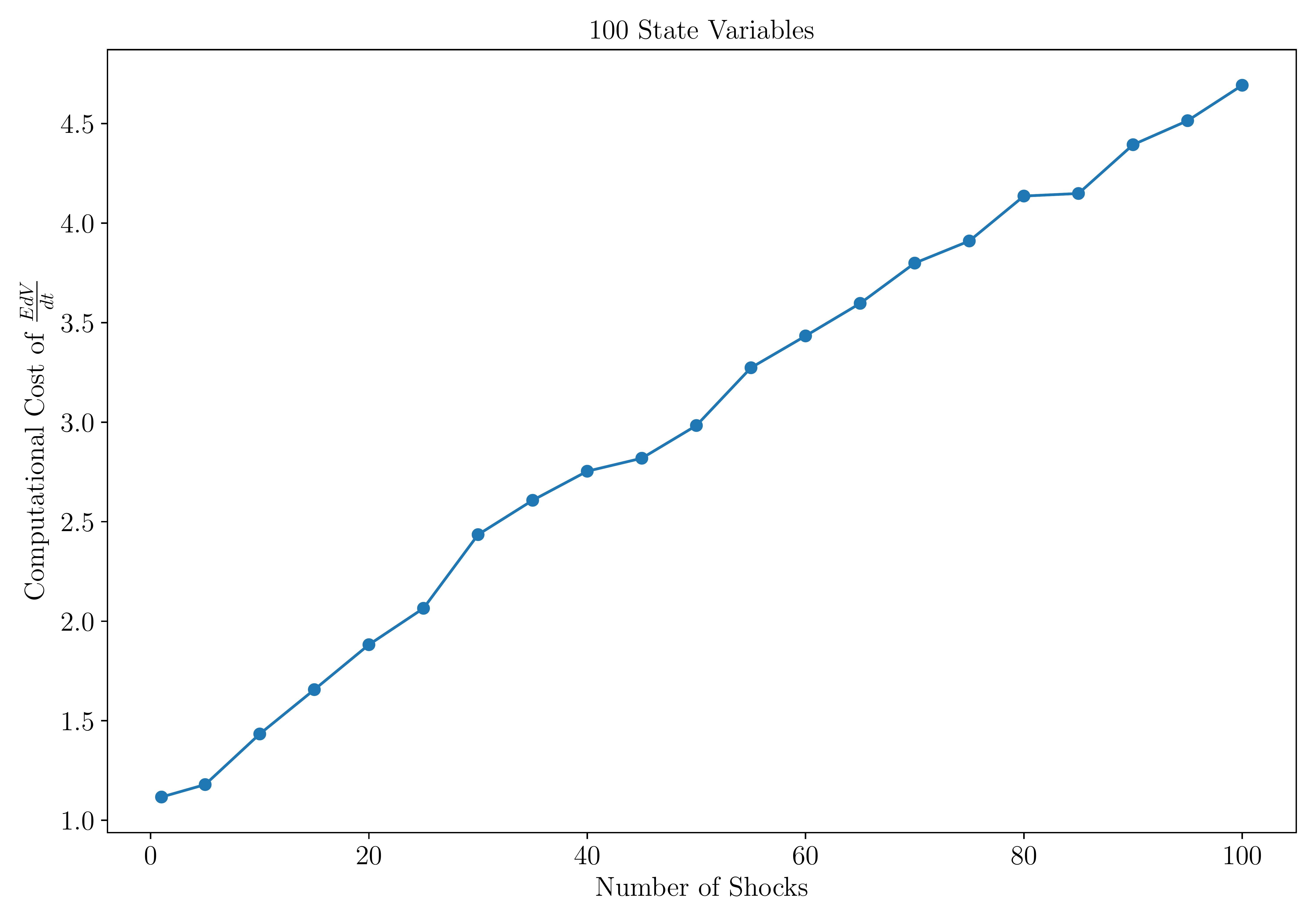
Notes: Cost is measured as the execution time of \(\frac{\mathbb{E}dV}{dt}(\mathbf{s})\) relative to that of \(V(\mathbf{s})\). The left panel fixes \(m=1\) and varies \(n\) from 1 to 100; the right panel fixes \(n=100\) and varies \(m\) from 1 to 100. In this example, \(V\) is a two-layer neural network, and execution times are averaged over 10,000 runs on a mini-batch of 512 states.

Computational Cost (continued)

We benchmark the performance of the hyper-dual approach to Itô’s lemma by comparing the execution time of alternative methods.

• In addition to finite differences and naive autodiff, we also consider the analytical expression for the derivatives

The hyper-dual Itô’s lemma method is faster and less memory-intensive than using the analytical expression for the derivatives.

Method	FLOPs	Memory	Error
1. Finite differences	9,190,800	112,442,048	1.58%
2. Naive autodiff	2,100,501	25,673,640	0.00%
3. Analytical	20,501	44,428	0.00%
4. Hyper-dual Itô	599	6,044	0.00%

III. The Deep Policy Iteration Algorithm

Overcoming the Curse of Representation

Our objective is to compute the value function \(V(\mathbf{s})\) and policy function \(\mathbf{c}(\mathbf{s})\) satisfying the coupled functional equations: \[ 0 = \operatorname{HJB}(\mathbf{s}, \mathbf{c}(\mathbf{s}), V(\mathbf{s})), \qquad \mathbf{c}(\mathbf{s}) = \arg \max_{\mathbf{c}\in\Gamma(\mathbf{s})} \operatorname{HJB}(\mathbf{s},\mathbf{c},V(\mathbf{s})), \] where \[ \operatorname{HJB}(\mathbf{s},\mathbf{c},V) = u(\mathbf{c}) - \rho V + \nabla_{\mathbf{s}} V(\mathbf{s}) \cdot \mathbf{f}(\mathbf{s},\mathbf{c}) + \tfrac{1}{2} \operatorname{Tr}(\mathbf{g}(\mathbf{s},\mathbf{c}) \mathbf{H}_{\mathbf{s}} V(\mathbf{s}) \mathbf{g}(\mathbf{s},\mathbf{c})), \] and \(\mathbf{f}(\mathbf{s},\mathbf{c})\) is the drift of \(\mathbf{s}\) and \(\mathbf{g}(\mathbf{s},\mathbf{c})\) is the diffusion matrix.

To solve for \(V(\mathbf{s})\) and \(\mathbf{c}(\mathbf{s})\) numerically, we must represent them on a computer.

• A traditional approach is to discretize the state space and interpolate between grid points.

• In Module 4, we showed that such grid-based approximations can be viewed as shallow neural networks with fixed breakpoints.

Neural networks generalize this idea

• It allows us to learn flexible breakpoints and nonlinear combinations of basis functions.
• A DNN can approximate complex value and policy functions with relatively few parameters.

Overcoming the Curse of Optimization

We now turn to the challenge of training the DNNs to satisfy the functional equations above.

• A key difficulty lies in performing the maximization step efficiently, without resorting to costly root-finding procedures.

Our approach builds on generalized policy iteration (see, e.g., Sutton and Barto (2018))

• Combining with deep function approximation, alternating between policy evaluation and policy improvement.

• This leads to the Deep Policy Iteration (DPI) algorithm.

The algorithm proceeds in three stages:

1. Sampling
2. Policy improvement
3. Policy evaluation

Simplifying assumptions.

For clarity, we make several simplifying assumptions that can be relaxed in practice.

1. We adopt plain stochastic gradient descent (SGD) for parameter updates.
2. We perform exactly one iteration of policy evaluation and policy improvement at each update.
3. We use a quadratic loss function for the policy evaluation step.

Step 1: Sampling

We begin by sampling a mini-batch of states \(\{\mathbf{s}_i\}_{i=1}^I\) from the state space.

• This can be done using a uniform distribution within plausible state-space bounds.
• Alternatively, we can use an estimated ergodic distribution based on previous iterations.

Step 2: Policy Improvement

The policy improvement step involves solving the maximization step for each state in the mini-batch.

• This step can be computationally demanding and lies at the heart of the curse of optimization.

Generalized policy iteration.

In Module 3, we introduced the policy function iteration, which alternates between policy evaluation and policy improvement steps.

• In the policy evaluation step, we solve for the new value function \(V_{n+1}(\mathbf{s})\) given the policy \(\mathbf{c}_n(\mathbf{s})\).
• In the policy improvement step, we solve for the new policy \(\mathbf{c}_{n+1}(\mathbf{s})\) given the current value function \(V_{n+1}(\mathbf{s})\).

However, when the initial guess for \(V\) is far from optimal, fully solving the maximization problem at each iteration is inefficient.

• This motivates an approximate policy improvement step that performs only a single gradient-based update in the direction of improvement.

Fix the current parameter vectors for the value and policy functions, \(\mathbf{\theta}_V^{j-1}\) and \(\mathbf{\theta}_C^{j-1}\).

• Evaluate the value and policy functions at the mini-batch of states: \(V_{j-1,i} = V(\mathbf{s}_i; \mathbf{\theta}_V^{j-1})\) and \(\mathbf{c}_{j-1,i} = \mathbf{c}(\mathbf{s}_i; \mathbf{\theta}_C^{j-1})\).
• We can use the \(\{\mathbf{s}_i, V_{j-1,i},\mathbf{c}_{j-1,i}\}_{i=1}^I\) as a training data to update the policy function.

Step 2: Policy Improvement (continued)

Our goal is to choose the policy function to maximize (or minimize minus) the value of the HJB operator

• We can then define the loss function as follows: \[ \mathcal{L}_p(\mathbf{\theta}_C) = - \frac{1}{2I}\sum_{i=1}^I \operatorname{HJB}(\mathbf{s}_i, \mathbf{\theta}_{C}^{j-1}, \mathbf{\theta}_{V}^{j-1}), \] where \(\operatorname{HJB}(\mathbf{s}_i, \mathbf{\theta}_{C}^{j-1}, \mathbf{\theta}_{V}^{j-1}) \equiv \operatorname{HJB}(\mathbf{s}_i, \mathbf{c}_{j-1,i}, V_{j-1,i})\).

We perform one step of gradient descent on the loss function to update the policy function parameters:

Policy improvement step.

\[\begin{equation}\label{eq:policy_improvement_step} \mathbf{\theta}_C^{j} = \mathbf{\theta}_C^{j-1} + \eta_C \frac{1}{I}\sum_{i=1}^I \nabla_{\mathbf{\theta}_C} \operatorname{HJB}(\mathbf{s}_i, \mathbf{\theta}_C^{j-1}, \mathbf{\theta}_V^{j-1}), \end{equation}\]

where \(\eta_C\) is the learning rate controlling the step size in parameter space.

Step 3: Policy Evaluation I

We now update the value function given the new policy parameters, \(\mathbf{\theta}_C^{j}\).

• We present two alternative update rules, each with distinct trade-offs.

The first rule mirrors the explicit method for finite-differences in Module 3.

• Consider a false-transient formulation that iterates the value function backward in (pseudo-)time:

\[ \frac{V(\mathbf{s}; \mathbf{\theta}_V^{j}) - V(\mathbf{s}_i; \mathbf{\theta}_V^{j-1})}{\Delta t} = \operatorname{HJB}(\mathbf{s}_i, \mathbf{\theta}_C^{j}, \mathbf{\theta}_V^{j-1}) \qquad \Rightarrow \qquad V(\mathbf{s}; \mathbf{\theta}_V^{j}) = \underbrace{V(\mathbf{s}_i; \mathbf{\theta}_V^{j-1}) + \operatorname{HJB}(\mathbf{s}_i, \mathbf{\theta}_C^{j}, \mathbf{\theta}_V^{j-1}) \Delta t}_{\text{target value } \hat{V}_i^{j-1}}, \] where the HJB is evaluated at the new policy parameters, \(\mathbf{\theta}_C^{j}\), but old value function parameters, \(\mathbf{\theta}_V^{j-1}\).

This turns the problem into a supervised learning task given the training data \(\{\mathbf{s}_i, \hat{V}_i^{j-1}\}_{i=1}^I\).

Step 3: Policy Evaluation I (continued)

Define the loss function as the mean-squared error between the target value and the value function: \[ \mathcal{L}(\mathbf{\theta}_V) = \frac{1}{2I}\sum_{i=1}^I (V(\mathbf{s}_i; \mathbf{\theta}_V) - \hat{V}_i^{j-1})^2, \]

Evaluating the gradient at \(\mathbf{\theta}_V^{j-1}\) yields \[ \nabla_{\mathbf{\theta}_V} \mathcal{L}(\mathbf{\theta}_V^{j-1}) = -\frac{\Delta t}{I}\sum_{i=1}^I \operatorname{HJB}(\mathbf{s}_i, \mathbf{\theta}_C^{j}, \mathbf{\theta}_V^{j-1}) \nabla_{\mathbf{\theta}_V} V(\mathbf{s}_i; \mathbf{\theta}_V), \]

Taking one step of gradient descent, the corresponding update rule is:

Policy evaluation step.

\[ \mathbf{\theta}_V^{j} = \mathbf{\theta}_V^{j-1} + \eta_V \frac{\Delta t}{I}\sum_{i=1}^I \operatorname{HJB}(\mathbf{s}_i, \mathbf{\theta}_C^{j}, \mathbf{\theta}_V^{j-1}) \nabla_{\mathbf{\theta}_V} V(\mathbf{s}_i; \mathbf{\theta}_V^{j-1}), \]

where \(\eta_V\) is the learning rate.

Step 3: Policy Evaluation II

The second rule mirrors the implicit method for finite-differences in Module 3: \[ \frac{V(\mathbf{s}; \mathbf{\theta}_V^{j}) - V(\mathbf{s}_i; \mathbf{\theta}_V^{j-1})}{\Delta t} = \operatorname{HJB}(\mathbf{s}_i, \mathbf{\theta}_C^{j}, \mathbf{\theta}_V^{j}), \] As in the implicit finite-difference method, we can take the limit as \(\Delta t \to \infty\).

In this case, the loss function becomes MSE of HJB residuals: \[ \mathcal{L}(\mathbf{\theta}_V) = \frac{1}{2I}\sum_{i=1}^I \operatorname{HJB}(\mathbf{s}_i, \mathbf{\theta}_C^{j}, \mathbf{\theta}_V)^2, \]

The gradient is given by \[ \nabla_{\mathbf{\theta}_V} \mathcal{L}(\mathbf{\theta}_V) = \frac{1}{I}\sum_{i=1}^I \operatorname{HJB}(\mathbf{s}_i, \mathbf{\theta}_C^{j}, \mathbf{\theta}_V) \nabla_{\mathbf{\theta}_V} \operatorname{HJB}(\mathbf{s}_i, \mathbf{\theta}_C^{j}, \mathbf{\theta}_V), \]

Evaluating at \(\mathbf{\theta}_V^{j-1}\) yields

Policy evaluation step 2.

\[ \mathbf{\theta}_V^{j} = \mathbf{\theta}_V^{j-1} - \eta_V \frac{1}{I}\sum_{i=1}^I \operatorname{HJB}(\mathbf{s}_i, \mathbf{\theta}_C^{j}, \mathbf{\theta}_V^{j-1}) \nabla_{\mathbf{\theta}_V} \operatorname{HJB}(\mathbf{s}_i, \mathbf{\theta}_C^{j}, \mathbf{\theta}_V^{j-1}), \]

where \(\eta_V\) is the learning rate.

The Deep Policy Iteration Algorithm

We can now summarize the complete algorithm:

Algorithm: Deep Policy Iteration (DPI)

Input: Initial parameters \(\mathbf{\theta}_V^{0}\) and \(\mathbf{\theta}_C^{0}\)

Output: Value function \(V(\mathbf{s}; \mathbf{\theta}_V)\), policy function \(\mathbf{c}(\mathbf{s}; \mathbf{\theta}_C)\)

Initialize: \(j \gets 0\)

Repeat for \(j = 1, 2, \ldots\):

1. Sampling:
   Sample a mini-batch of states \(\{\mathbf{s}_i\}_{i=1}^I\).

2. Policy improvement (actor update):
   Update \(\mathbf{\theta}_C\) with one step of gradient descent on the loss function.

3. Policy evaluation (critic update):
   Update \(\mathbf{\theta}_V\) using the explicit or implicit policy evaluation step.

The trade-off between the two update rules.

Minimizing the Bellman residual directly is known to be more stable but it is often slower than iterative policy evaluation.

• Moreover, the implicit policy evaluation step requires relatively costly third-order derivatives, since \(\nabla_{\mathbf{\theta}_V} \operatorname{HJB}(\mathbf{s}_i, \mathbf{\theta}_C^{j}, \mathbf{\theta}_V)\) involves the Hessian of \(V\).
• As a rule of thumb, it is preferable to start with the explicit policy evaluation step for speed, and switch to the implicit policy evaluation step if necessary.

IV. Applications: Asset Pricing

Asset Pricing: The Two-Trees Model

Next, we apply the DPI algorithm to solve a variety of economic and financial problems.

• We focus on three canonical domains of finance: asset pricing, corporate finance, and portfolio choice.
• We illustrate how the DPI algorithm can be applied to solve a variety of economic and financial problems.

To start, we consider the familiar two-trees model from Module 3.

The pricing condition for a log investor implies \[ v_t = \mathbb{E}_t \left[ \int_{0}^{\infty} e^{-\rho s} s_{t+s}\,ds \right], \] where the relative share process \(s_t\) evolves as \[ d s_t = - 2 \sigma^2 s_t(1-s_t)\!\left(s_t - \tfrac12\right) dt + \sigma s_t(1-s_t)(dB_{1,t} - dB_{2,t}). \]

The price-consumption ratio \(v_t\) satisfies the HJB equation: \[ \rho v = s - v_s \, 2\sigma^2 s(1-s)\!\left(s-\tfrac12\right) + \frac{1}{2} v_{ss}\,\big(2\sigma^2 s^2(1-s)^2\big), \] with boundary conditions \(v(0) = 0\) and \(v(1) = 1/\rho\).

It is straightforward to solve this one-dimensional problem using finite differences or collocation methods

• But we solve it here using the DPI framework to illustrate the workflow.

Julia Implementation

We now implement the two-trees model in Julia, starting with the model struct.

@kwdef struct TwoTrees
    ρ::Float64 = 0.04
    σ::Float64 = sqrt(0.04)
    μ::Float64 = 0.02
    μₛ::Function = s -> @. -2 * σ^2 * s * (1-s) * (s-0.5)   # drift of s
    σₛ::Function = s -> @. sqrt(2) * σ * s * (1-s)          # diffusion of s
end;

m = TwoTrees()

TwoTrees(0.04, 0.2, 0.02, var"#6#10"{Float64}(0.2), var"#7#11"{Float64}(0.2))

We next implement the hyper-dual approach to Ito’s lemma to compute the drift and diffusion of the state variable \(s\).

using ForwardDiff
function drift_hyper(V::Function, s::AbstractMatrix, m::TwoTrees)
    F(ϵ) = V(s + m.σₛ(s)/sqrt(2)*ϵ + m.μₛ(s)/2*ϵ^2)
    return ForwardDiff.derivative(ϵ -> ForwardDiff.derivative(F, ϵ), 0.0)
end;

To validate the implementation, we can compare the analytical and hyper-dual drifts:

using Random
rng = Xoshiro(0)  
s   = rand(rng, 1, 1000)
# Exact drift for test function
V_test(s) = sum(s.^2, dims = 1)
drifts_exact = map(1:size(s, 2)) do i
    ∇V, H = 2 * s[:,i], 2 * Matrix(I,length(s[:,i]),length(s[:,i]))
    ∇V' * m.μₛ(s[:,i]) + 0.5 * tr(m.σₛ(s[:,i])' * H * m.σₛ(s[:,i]))
end'
drifts_hyper = drift_hyper(V_test, s, m)
errors = maximum(abs.(drifts_exact - drifts_hyper))

1.734723475976807e-18

Neural Network Implementation

We now implement the neural network representation of the value function.

using Lux
model = Chain(
    Dense(1 => 25, Lux.gelu),
    Dense(25 => 25, Lux.gelu),
    Dense(20 => 1)
)

Chain(
    layer_1 = Dense(1 => 25, gelu_tanh),          # 50 parameters
    layer_2 = Dense(25 => 25, gelu_tanh),         # 650 parameters
    layer_3 = Dense(20 => 1),                     # 21 parameters
)         # Total: 721 parameters,
          #        plus 0 states.

We initialize the parameters and optimizer state using the Adam optimizer with a learning rate of \(10^{-3}\).

using Optimisers
rng = Xoshiro(0)
ps, ls = Lux.setup(rng, model) |> f64
opt = Adam(1e-3)
os = Optimisers.setup(opt, ps)

(layer_1 = (weight = Leaf(Adam(eta=0.001, beta=(0.9, 0.999), epsilon=1.0e-8), ([0.0; 0.0; … ; 0.0; 0.0;;], [0.0; 0.0; … ; 0.0; 0.0;;], (0.9, 0.999))), bias = Leaf(Adam(eta=0.001, beta=(0.9, 0.999), epsilon=1.0e-8), ([0.0, 0.0, 0.0, 0.0, 0.0, 0.0, 0.0, 0.0, 0.0, 0.0  …  0.0, 0.0, 0.0, 0.0, 0.0, 0.0, 0.0, 0.0, 0.0, 0.0], [0.0, 0.0, 0.0, 0.0, 0.0, 0.0, 0.0, 0.0, 0.0, 0.0  …  0.0, 0.0, 0.0, 0.0, 0.0, 0.0, 0.0, 0.0, 0.0, 0.0], (0.9, 0.999)))), layer_2 = (weight = Leaf(Adam(eta=0.001, beta=(0.9, 0.999), epsilon=1.0e-8), ([0.0 0.0 … 0.0 0.0; 0.0 0.0 … 0.0 0.0; … ; 0.0 0.0 … 0.0 0.0; 0.0 0.0 … 0.0 0.0], [0.0 0.0 … 0.0 0.0; 0.0 0.0 … 0.0 0.0; … ; 0.0 0.0 … 0.0 0.0; 0.0 0.0 … 0.0 0.0], (0.9, 0.999))), bias = Leaf(Adam(eta=0.001, beta=(0.9, 0.999), epsilon=1.0e-8), ([0.0, 0.0, 0.0, 0.0, 0.0, 0.0, 0.0, 0.0, 0.0, 0.0  …  0.0, 0.0, 0.0, 0.0, 0.0, 0.0, 0.0, 0.0, 0.0, 0.0], [0.0, 0.0, 0.0, 0.0, 0.0, 0.0, 0.0, 0.0, 0.0, 0.0  …  0.0, 0.0, 0.0, 0.0, 0.0, 0.0, 0.0, 0.0, 0.0, 0.0], (0.9, 0.999)))), layer_3 = (weight = Leaf(Adam(eta=0.001, beta=(0.9, 0.999), epsilon=1.0e-8), ([0.0 0.0 … 0.0 0.0], [0.0 0.0 … 0.0 0.0], (0.9, 0.999))), bias = Leaf(Adam(eta=0.001, beta=(0.9, 0.999), epsilon=1.0e-8), ([0.0], [0.0], (0.9, 0.999)))))

We define the loss function as the mean-squared error between the value function and the target value.

loss_fn(ps, ls, s, target) = mean(abs2, model(s, ps, ls)[1] - target)

# Target value function
function target(v, s, m; Δt = 0.2)
    hjb = s + drift_hyper(v, s, m) - m.ρ * v(s)
    return v(s) + hjb * Δt
end;

Training the Neural Network

We now train the neural network using the Adam optimizer.

# Training loop
loss_history = Float64[]
for i = 1:40_000
    s_batch = rand(rng, 1,  128)
    tgt     = target(s-> model(s, ps, ls)[1], s_batch, m, Δt = 1.0)
    loss    = loss_fn(ps, ls, s_batch, tgt)
    grad    = gradient(p -> loss_fn(p, ls, s_batch, tgt), ps)[1]
    os, ps  = Optimisers.update(os,ps, grad)
    push!(loss_history, loss)
end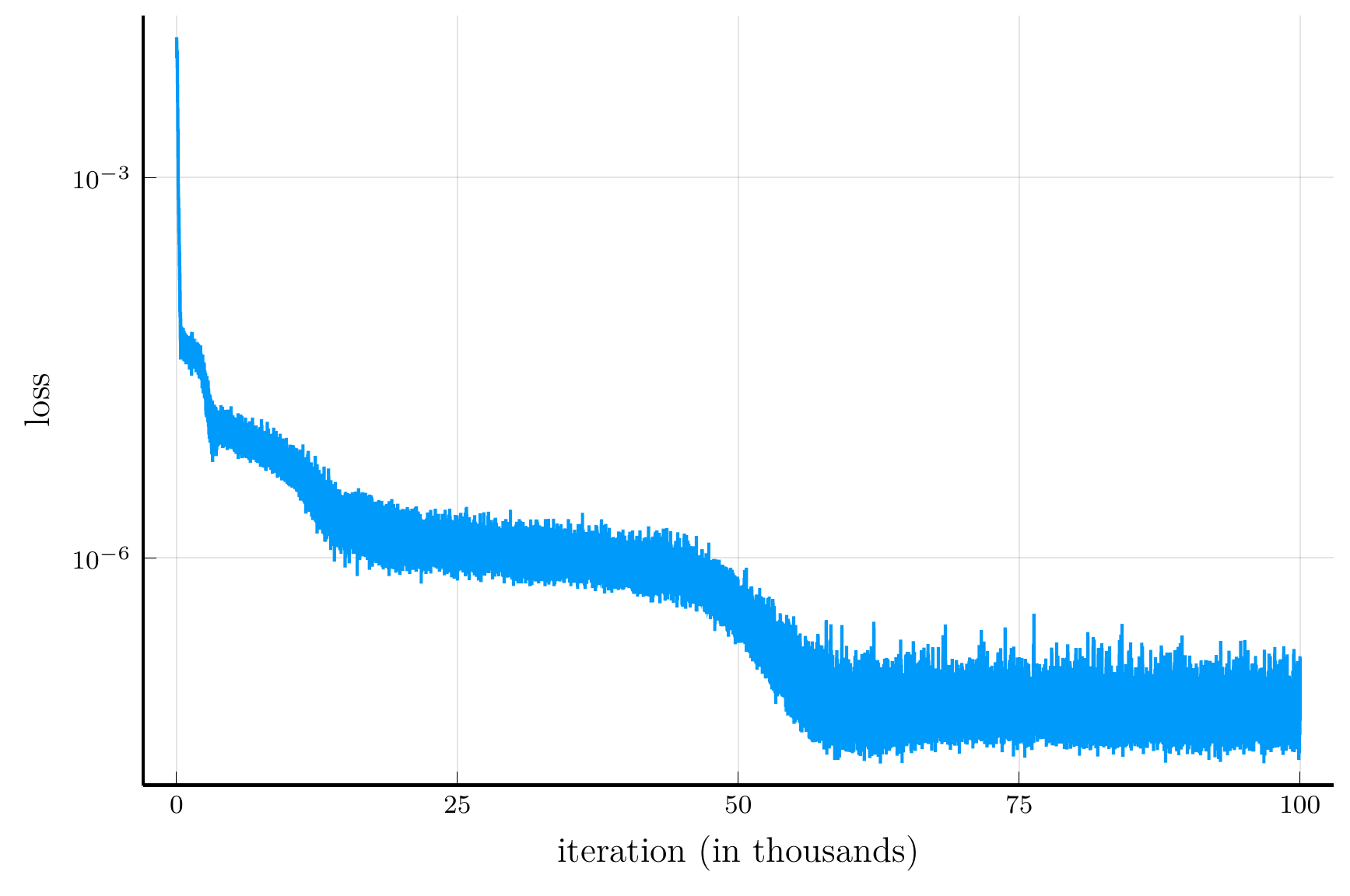

Training loss over iterations.

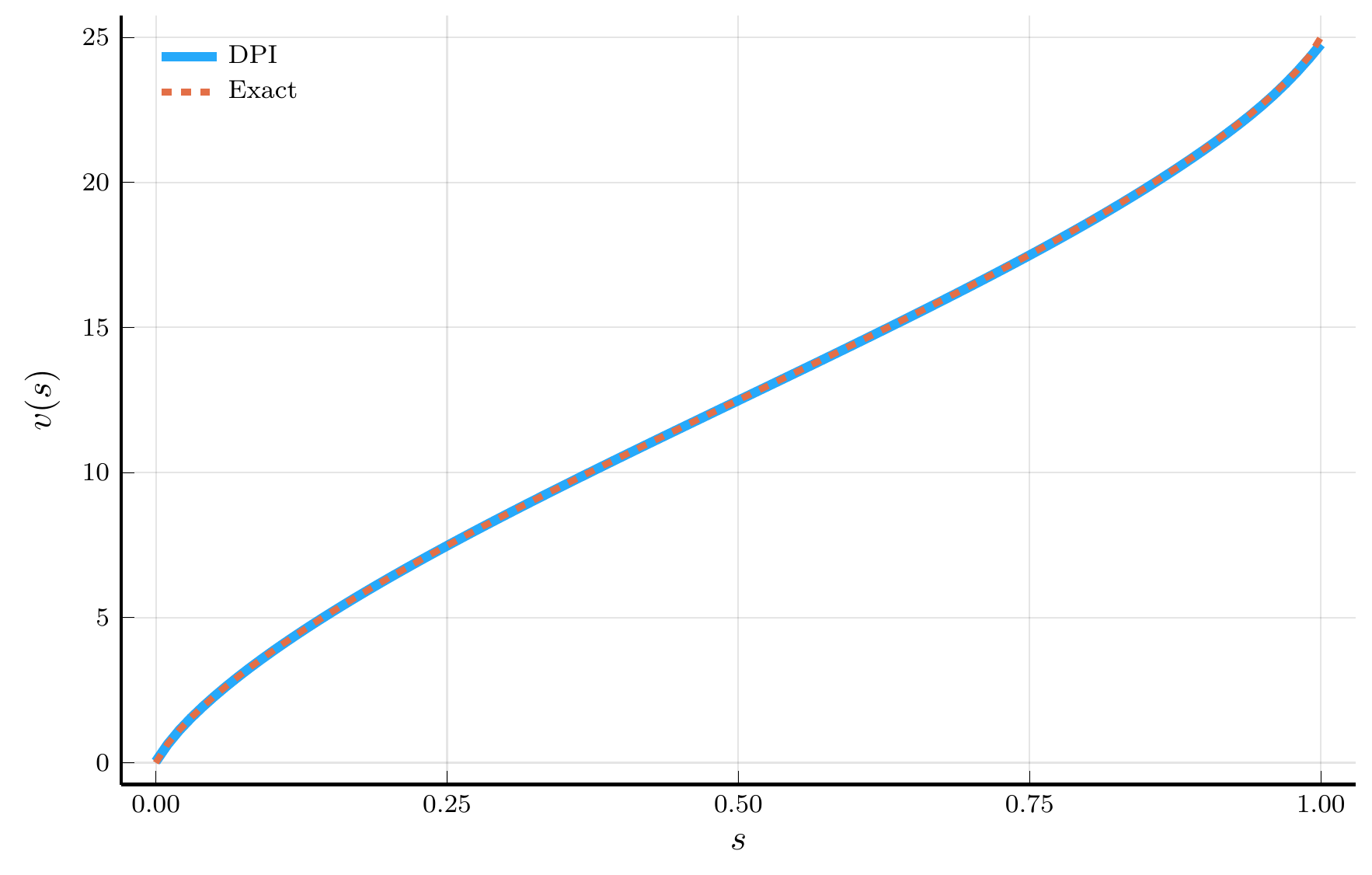
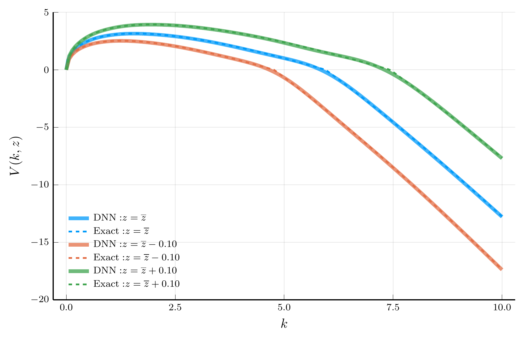
DPI prediction vs. analytical solution.

The Lucas Orchard Model

We now extend the two-trees model to a multi-tree economy, known as the Lucas orchard model (see, e.g., Martin (2013)).

• By varying the number of trees, we can examine how the DPI algorithm scales with the dimensionality of the state space.

Consider a representative investor with log utility who can invest in a riskless asset and \(N\) risky assets.

• Each risky asset \(i\) pays a continuous dividend stream \(D_{i,t}\) that follows a geometric Brownian motion: \[ \frac{d D_{i,t}}{D_{i,t}} = \mu_i\,dt + \sigma_i\,dB_{i,t}, \] where each \(B_{i,t}\) is a Brownian motion satisfying \(dB_{i,t}\,dB_{j,t} = 0\) for \(i \neq j\).

The HJB equation.

Define the vector of state variables \(\mathbf{s}_t = (s_{1,t}, \ldots, s_{N,t})^{\!\top}\), where \(s_{i,t} \equiv D_{i,t}/C_t\) and \(C_t = \sum_{i=1}^N D_{i,t}\).

• Let \(v_{i,t} \equiv P_{i,t}/C_t\) denote the price–consumption ratio of asset \(i\).
• The pricing condition for a log investor implies \[ \rho\,v_i(\mathbf{s}) = s_i + \nabla_{\mathbf{s}} v_i(\mathbf{s})^{\!\top} \mathbf{\mu}_s(\mathbf{s}) + \frac{1}{2}\operatorname{Tr}\!\left[ \mathbf{\sigma}_s(\mathbf{s})^{\!\top} \mathbf{H}_{\mathbf{s}} v_i(\mathbf{s}) \mathbf{\sigma}_s(\mathbf{s}) \right] \] subject to the boundary conditions \(v_i(0) = 0\) and \(v_i(1) = 1/\rho\).

Julia Implementation

We now implement the Lucas orchard model in Julia.

• The workflow of the DPI algorithm for the Lucas orchard model is virtually identical to that for the simple two-trees model.

As usual, we start by defining the model struct.

@kwdef struct LucasOrchard
    ρ::Float64 = 0.04
    N::Int = 10
    σ::Vector{Float64} = sqrt(0.04) * ones(N)
    μ::Vector{Float64} = 0.02 * ones(N)
    μc::Function = s -> μ' * s
    σc::Function = s -> [s[i,:]' * σ[i] for i in 1:N]
    μₛ::Function = s ->  s .* (μ .- μc(s)- s.*σ.^2 .+ sum(σc(s)[i].^2 for i in 1:N))
    σₛ::Function = s -> [s .* ([j == i ? σ[i] : 0 for j in 1:N] .- σc(s)[i]) for i in 1:N] 
end;

# Instantiate the model
using Distributions, Random
m         = LucasOrchard(N = 10) # number of assets
rng, d    = MersenneTwister(0), Dirichlet(ones(m.N)) # Dirichlet distribution
s_samples = rand(rng, d, 1_000) # N x 1_000 matrix
m.μₛ(s_samples) # N x 1_000 matrix

10×1000 Matrix{Float64}:
  4.24309e-5    0.000237275   0.000815818  …   8.57681e-5   -0.00169363
 -0.000259516   0.000134325   0.000132953      0.000550971   0.000463926
  0.000193812   0.000154873   0.000418759      0.000564647   5.89399e-5
  0.000118302   0.00023403   -0.00379805       2.65856e-5    0.000710309
  0.000187861   0.000109689   0.000126233      0.000119859  -0.00071501
 -2.52101e-6    4.92026e-5    0.000566168  …   0.00054645    0.000122228
  0.000199586   4.887e-6      7.50461e-5       0.000573028   0.000189173
  2.76043e-5   -0.000877846   0.000535931      0.000335935   0.00040788
 -0.000704084  -9.64787e-5    0.000686905     -0.00331773    0.000103212
  0.000196524   5.00425e-5    0.000440236      0.00051449    0.000352971

The Hyper-dual Approach to Ito’s Lemma

We next implement the hyper-dual approach to Ito’s lemma to compute the drift and diffusion of the state variable \(s\).

using ForwardDiff
function drift_hyper(V::Function, s::AbstractMatrix, m::LucasOrchard)
    N, σs, μs = m.N, m.σₛ(s), m.μₛ(s) # Preallocations
    F(ϵ) = sum(V(s .+ σs[i] .* (ϵ / sqrt(2)) .+ μs .* (ϵ^2 / (2 * N))) for i in 1:N)
    return ForwardDiff.derivative(ϵ -> ForwardDiff.derivative(F, ϵ), 0.0)
end;

The implementation is virtually identical to that for the two-trees model.

• But now we are dealing with the case of multiple state variables and Brownian motions.

The importance of preallocations.

Relative to the two-trees model, we now preallocate arrays for the drift and diffusion of the state variable \(s\),

• Instead of constructing them inside loops over \(i = 1, \ldots, N\).
• In higher-dimensional problems, preallocations avoid repeated memory allocation and garbage collection, improving performance.

Neural Network Implementation

We next implement the neural network representation of the value function.

• We use essentially the same architecture as in the two-trees model.
• But now the input is the \(N\)-dimensional vector of state variables \(\mathbf{s}_t\).

model = Chain(
    Dense(m.N => 25, Lux.gelu),
    Dense(25 => 25, Lux.gelu),
    Dense(25 => 1)
)

Chain(
    layer_1 = Dense(10 => 25, gelu_tanh),         # 275 parameters
    layer_2 = Dense(25 => 25, gelu_tanh),         # 650 parameters
    layer_3 = Dense(25 => 1),                     # 26 parameters
)         # Total: 951 parameters,
          #        plus 0 states.

We initialize the parameters and optimizer state using the Adam optimizer with a learning rate of \(10^{-3}\).

ps, ls = Lux.setup(rng, model) |> f64
opt = Adam(1e-3)
os = Optimisers.setup(opt, ps)

(layer_1 = (weight = Leaf(Adam(eta=0.001, beta=(0.9, 0.999), epsilon=1.0e-8), ([0.0 0.0 … 0.0 0.0; 0.0 0.0 … 0.0 0.0; … ; 0.0 0.0 … 0.0 0.0; 0.0 0.0 … 0.0 0.0], [0.0 0.0 … 0.0 0.0; 0.0 0.0 … 0.0 0.0; … ; 0.0 0.0 … 0.0 0.0; 0.0 0.0 … 0.0 0.0], (0.9, 0.999))), bias = Leaf(Adam(eta=0.001, beta=(0.9, 0.999), epsilon=1.0e-8), ([0.0, 0.0, 0.0, 0.0, 0.0, 0.0, 0.0, 0.0, 0.0, 0.0  …  0.0, 0.0, 0.0, 0.0, 0.0, 0.0, 0.0, 0.0, 0.0, 0.0], [0.0, 0.0, 0.0, 0.0, 0.0, 0.0, 0.0, 0.0, 0.0, 0.0  …  0.0, 0.0, 0.0, 0.0, 0.0, 0.0, 0.0, 0.0, 0.0, 0.0], (0.9, 0.999)))), layer_2 = (weight = Leaf(Adam(eta=0.001, beta=(0.9, 0.999), epsilon=1.0e-8), ([0.0 0.0 … 0.0 0.0; 0.0 0.0 … 0.0 0.0; … ; 0.0 0.0 … 0.0 0.0; 0.0 0.0 … 0.0 0.0], [0.0 0.0 … 0.0 0.0; 0.0 0.0 … 0.0 0.0; … ; 0.0 0.0 … 0.0 0.0; 0.0 0.0 … 0.0 0.0], (0.9, 0.999))), bias = Leaf(Adam(eta=0.001, beta=(0.9, 0.999), epsilon=1.0e-8), ([0.0, 0.0, 0.0, 0.0, 0.0, 0.0, 0.0, 0.0, 0.0, 0.0  …  0.0, 0.0, 0.0, 0.0, 0.0, 0.0, 0.0, 0.0, 0.0, 0.0], [0.0, 0.0, 0.0, 0.0, 0.0, 0.0, 0.0, 0.0, 0.0, 0.0  …  0.0, 0.0, 0.0, 0.0, 0.0, 0.0, 0.0, 0.0, 0.0, 0.0], (0.9, 0.999)))), layer_3 = (weight = Leaf(Adam(eta=0.001, beta=(0.9, 0.999), epsilon=1.0e-8), ([0.0 0.0 … 0.0 0.0], [0.0 0.0 … 0.0 0.0], (0.9, 0.999))), bias = Leaf(Adam(eta=0.001, beta=(0.9, 0.999), epsilon=1.0e-8), ([0.0], [0.0], (0.9, 0.999)))))

We define the loss function and the target function as before.

loss_fn(ps, ls, s, target) = mean(abs2, model(s, ps, ls)[1] - target)

# Target
function target(v, s, m; Δt = 0.2)
    v̅ = v(s)
    hjb = s[1,:]' + drift_hyper(v, s, m) - m.ρ * v̅
    return v̅ + hjb * Δt, mean(abs2, hjb)
end;

Training the Neural Network

# Training parameters
max_iter, Δt = 40_000, 1.0  
# Sampling interior and boundary states
d_int  = Dirichlet(ones(m.N))            # Interior region
d_edge = Dirichlet(0.05 .* ones(m.N))  # Boundary region
# Loss history and exponential moving average loss
loss_history, loss_ema_history, α_ema = Float64[], Float64[], 0.99
# Training loop
p = Progress(max_iter; desc="Training...", dt=1.0) #progress bar
for i = 1:max_iter
    if rand(rng) < 0.50
        s_batch = rand(rng, d_int, 128)
    else
        s_batch = rand(rng, d_edge, 128)
    end
    v(s)       = model(s, ps, ls)[1] # define value function
    tgt, hjb_res = target(v, s_batch, m, Δt = Δt) #target/residual
    loss, back = Zygote.pullback(p -> loss_fn(p,ls,s_batch,tgt), ps)
    grad       = first(back(1.0)) # gradient
    os, ps     = Optimisers.update(os,ps, grad) # update parameters
    loss_ema   = i==1 ? loss : α_ema*loss_ema + (1.0-α_ema)*loss
    push!(loss_history, loss)
    push!(loss_ema_history, loss_ema)
    next!(p, showvalues = [(:iter, i),("Loss", loss), 
        ("Loss EMA", loss_ema), ("HJB residual", hjb_res)])
end

We sample from two Dirichlet distributions:

• Interior region: uniform distribution over the simplex.
• Boundary region: highly concentrated near the edges.

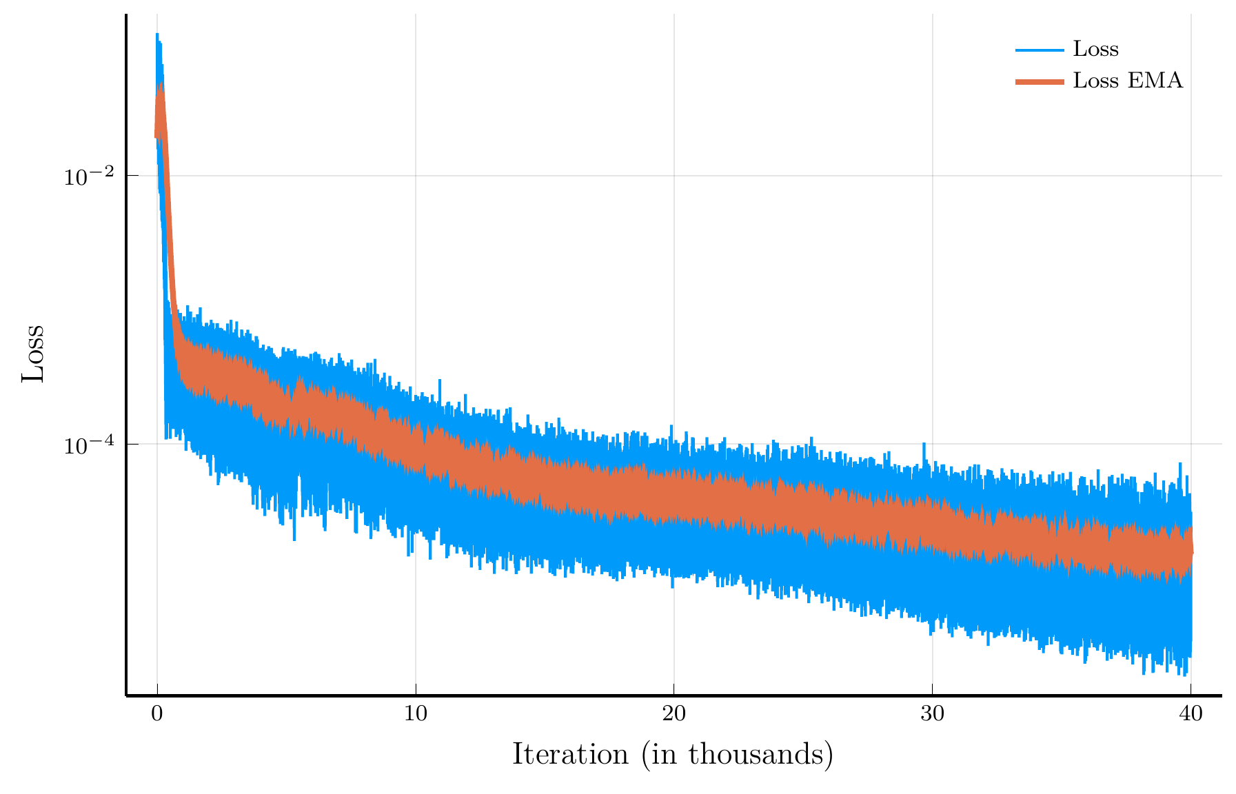
Training loss.

Test set evaluation I

We next evaluate the model’s performance on out-of-sample test sets.

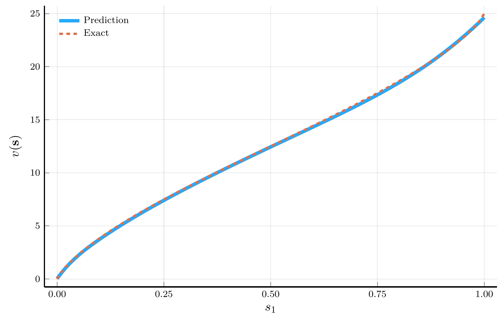
Two-trees prediction.

We consider an extremely asymmetric configuration:

• \(\mathbf{s} = (s_1, 1 - s_1, 0, \ldots, 0)\), the two-trees special case.
• This configuration lies outside the region used for training.

The network’s prediction replicates the analytical solution.

• Even though was not trained on this configuration,

Test set evaluation II

Our second test set draws states from a symmetric Dirichlet distribution with parameters \(\boldsymbol{\alpha} = \alpha_{\text{scale}} (1, 1, \ldots, 1)\)

• \(\alpha_{\text{scale}}\) controls the concentration of points within the simplex.
• Samples are concentrated near the center (or edges) of the simplex when \(\alpha_{\text{scale}} > 1\) (or \(< 1\)).

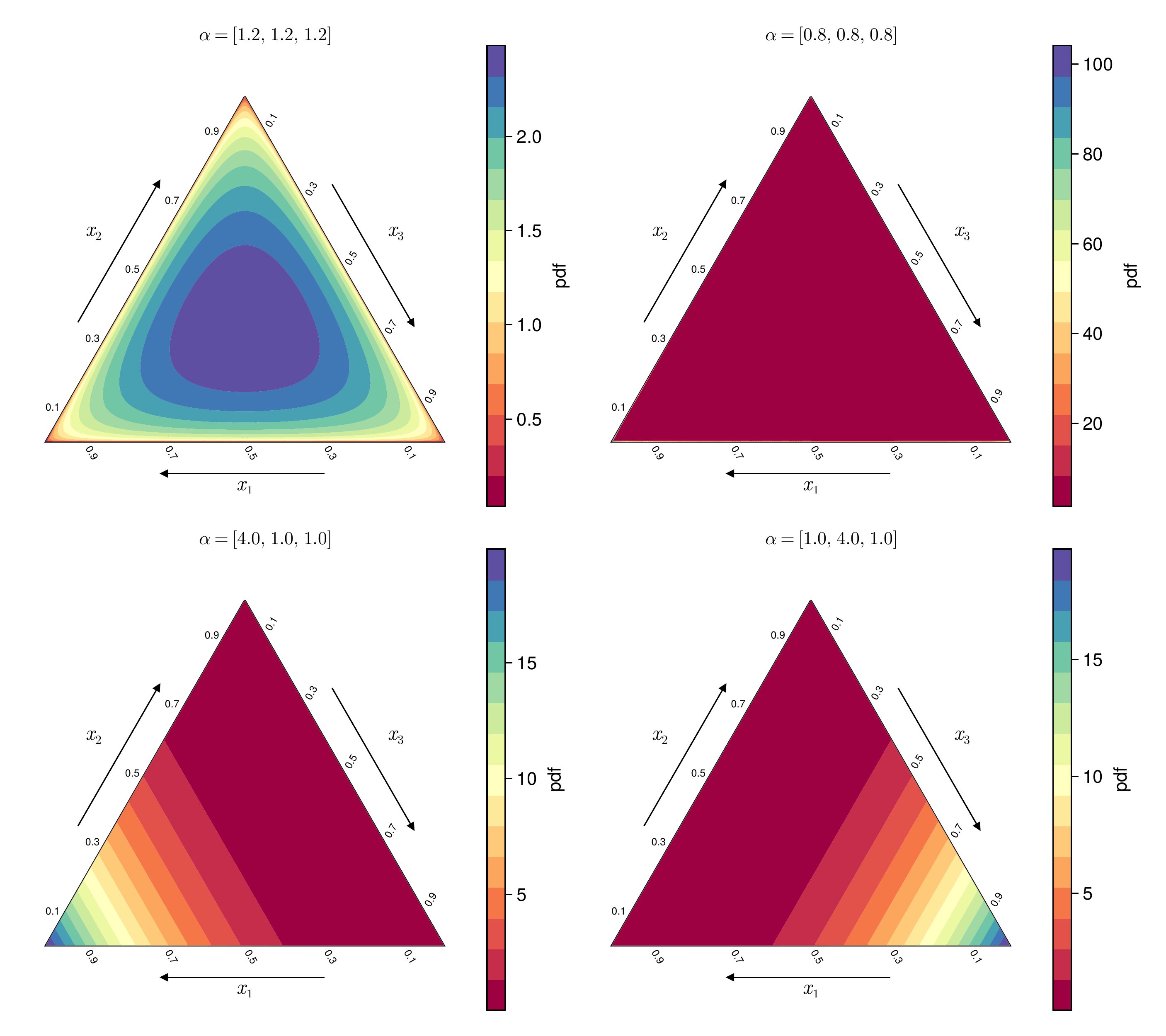
Dirichlet densities.

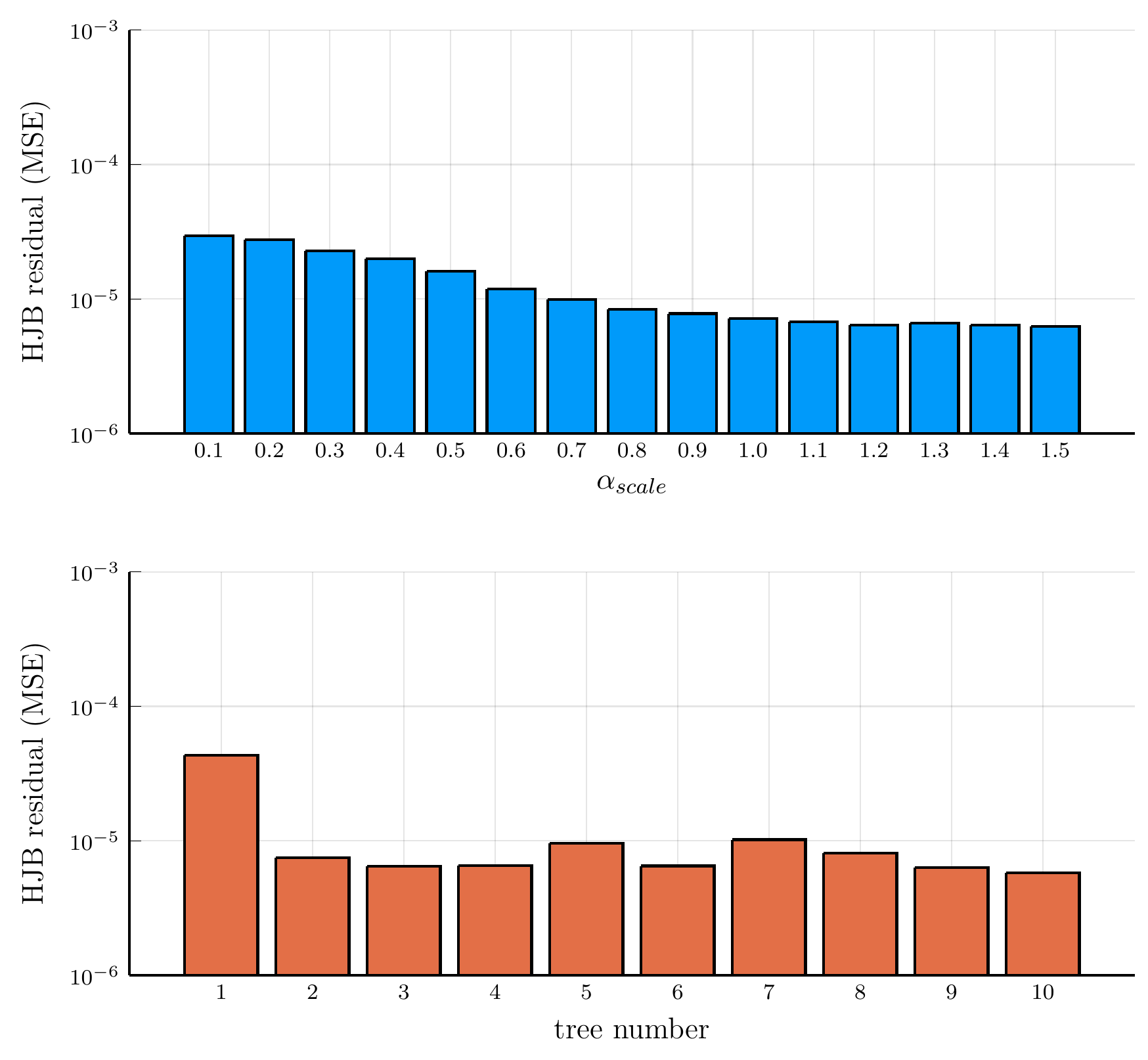
Orchard residuals.

Comparison with other methods

We next compare the DPI algorithm with other methods for solving high-dimensional dynamic models.

• We use the Lucas orchard model as a benchmark.

Finite-difference schemes become computationally infeasible beyond a few dimensions

• Chebyshev collocation on full tensor-product grids also suffers from exponential growth in cost.

We then compare the time to solution of the DPI algorithm with the Smolyak method (Smolyak (1963)).

• The Smolyak method is a sparse-grid technique for approximating multivariate functions
• It is commonly used for solving high-dimensional dynamic models.

Time to solution

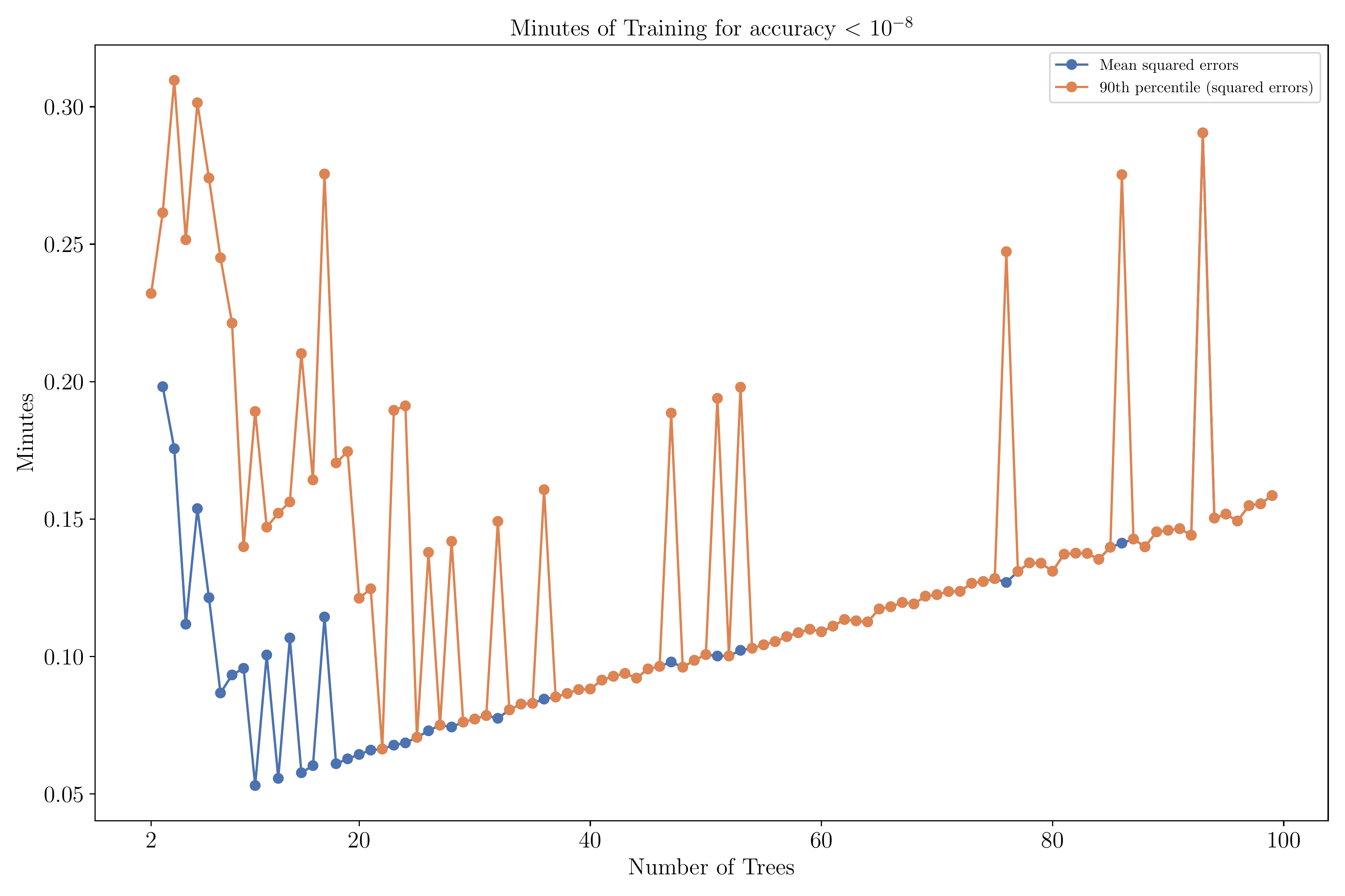
Notes: Figure shows the time-to-solution of the DPI algorithm, measured by the number of minutes required for the MSE or 90th-percentile squared error to fall below \(10^{-8}\). The parameter values are \(\rho = 0.04\), \(\gamma = 1\), \(\varrho = 0.0\), \(\mu = 0.015\), and \(\sigma = 0.1\). The HJB residuals are computed on a random sample of \(2^{13}\) points from the state space.

Smolyak vs. DPI algorithm

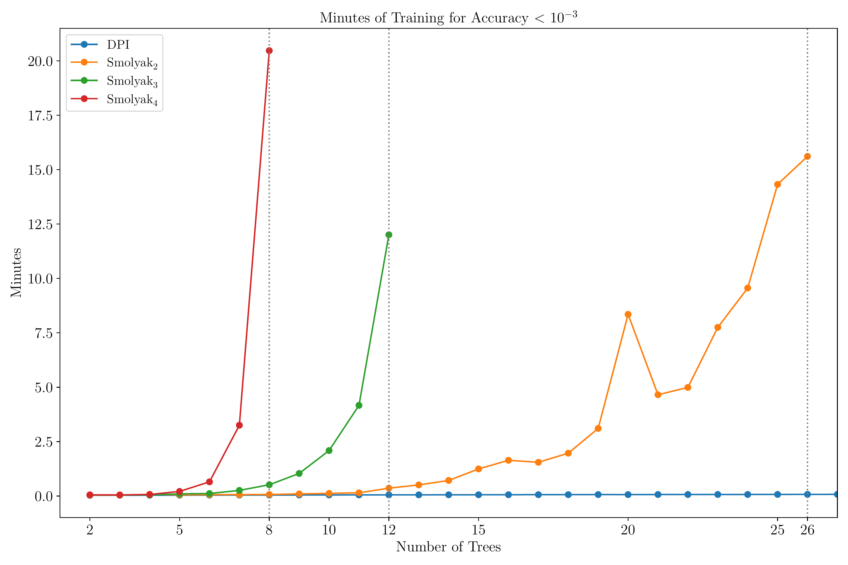
Notes: Figure compares the time-to-solution of the DPI method and the Smolyak methods of orders 2, 3, and 4. The tolerance is set to \(10^{-3}\), the highest accuracy threshold reached by all Smolyak variants. The parameter values are \(\rho = 0.04\), \(\gamma = 1\), \(\varrho = 0.0\), \(\mu = 0.015\), and \(\sigma = 0.1\). The HJB residuals are computed on a random sample of \(2^{13}\) points from the state space.

V. Applications: Corporate Finance

The Hennessy and Whited (2007) Model

We now apply the DPI algorithm to a corporate finance problem, a simplified version of the model in Hennessy and Whited (2007).

• This problem illustrates how the DPI algorithm can handle problems with kinks and inaction regions.

Consider a firm with operating profits \(\pi(k_t, z_t) = e^{z_t} k_t^\alpha\).

• Log productivity follows an Ornstein–Uhlenbeck process: \[ d z_t = -\theta (z_t - \bar{z})\,dt + \sigma\,dB_t, \] where \(\theta, \sigma > 0\).

• Given investment rate \(i_t\) and depreciation rate \(\delta\), capital evolves as \[ d k_t = (i_t - \delta)\,k_t\,dt. \]

The firm faces linear equity issuance costs \(\lambda > 0\).

• Operating profits net of adjustment costs are \[ D^*(k_t, z_t, i_t) = e^{z_t} k_t^\alpha - \left(i_t + 0.5 \chi i_t^2 \right) k_t, \] where \(\chi > 0\) is the adjustment cost parameter.

• The firm’s dividend policy is given by \[ D_t = D_t^* (1 + \lambda \mathbf{1}_{D_t^* < 0}). \]

The firm chooses the investment rate \(i_t\) to maximize the expected discounted value of future dividends: \[ v(\mathbf{s}_0) = \max_{\{i_t\}_{t\ge 0}} \mathbb{E}\left[ \int_{0}^{\infty} e^{-\rho s} D(k_s, z_s, i_s)\,ds \right], \] subject to the law of motion for the state vector \(\mathbf{s}_t = (k_t, z_t)^{\!\top}\).

The HJB Equation

The HJB equation is given by \[ 0 = \max_{i}\, \operatorname{HJB}(\mathbf{s}, i, v(\mathbf{s})), \] where \[ \operatorname{HJB}(\mathbf{s}, i, v) = D(k, z, i) + \nabla v^\top \mathbf{\mu}_{s}(\mathbf{s}, i) + \tfrac{1}{2}\,\mathbf{\sigma}_{s}(\mathbf{s}, i)^\top \mathbf{H}_{\mathbf{s}} v\, \mathbf{\sigma}_{s}(\mathbf{s}, i) - \rho v. \]

The first-order condition for the optimal investment rate is \[ \frac{\partial \operatorname{HJB}}{\partial i} = -\big(1 + \lambda\,\mathbf{1}_{D^*(k,z,i)<0}\big)\big[1 + \chi i \big]k + v_k(\mathbf{s})k = 0. \]

Consider a special case where there investment is fixed at \(i = \delta\) and productivity is constant \(\theta = \sigma = 0\).

• In this case, capital is constant
• From the HJB equation, we obtain the value function

\[ v(k, z) = \frac{D(k, z, \delta)}{\rho} = \begin{cases} \frac{e^{z} k^\alpha - \delta k}{\rho}, & \text{if } k \leq k_{\max}(z), \\[5pt] \frac{e^{z} k^\alpha - \delta k}{\rho} (1+\lambda), & \text{if } k > k_{\max}(z), \end{cases} \] where \(k_{\max}(z) = \left(\tfrac{e^{z}}{\delta}\right)^{\!\frac{1}{1-\alpha}}\).

Model struct and loss function

We start by defining the model struct.

@kwdef struct HennessyWhited
    α::Float64 = 0.55
    θ::Float64 = 0.26
    z̅::Float64 = 0.0
    σz::Float64 = 0.123
    δ::Float64 = 0.1
    χ::Float64 = 0.1
    λ::Float64 = 0.059
    ρ::Float64 = -log(0.96)
    μₛ::Function = (s,i) -> vcat((i .- δ) .* s[1,:]', -θ .* (s[2,:] .- z̅)')
    σₛ::Function = (s,i) -> vcat(zeros(1,size(s,2)), σz*ones(1,size(s,2)))
end;

The HJB is particularly simple in this case.

function hjb_special_case(m, s, θᵥ)
    (; α, λ, ρ, δ) = m
    k, z  = s[1,:]', s[2,:]'
    D_star     = exp.(z) .* k.^α - δ * k
    D     = D_star .* (1 .+ λ * (D_star .< 0))
    hjb   = D - ρ * v_net(s, θᵥ)
    return hjb
end

Given the HJB residual, we can define the loss function.

function loss_v_special_case(m, s, θᵥ)
    hjb = hjb_special_case(m, s, θᵥ)
    return mean(abs2, hjb)
end

Network architecture and training

We use a simple feedforward network with two hidden layers.

v_core = Chain(
    Dense(2, 32, Lux.swish),
    Dense(32, 24, Lux.swish),
    Dense(24, 1)
)

To enforce the boundary condition, we multiply the network by a function of \(k\) that vanishes at zero.

• A convenient choice is \(g(k) = k^\alpha\).

v_net(s, θᵥ) = (s[1,:].^m.α)' .* v_core(s, θᵥ, stᵥ)[1]

We initialize the parameters, optimizer, and training parameters.

# Initialize the parameters and optimizer
rng                  = Xoshiro(1234)
θᵥ, stᵥ              = Lux.setup(rng, v_core) |> Lux.f64
optᵥ                 = Optimisers.Adam(1e-3)
osᵥ                  = Optimisers.setup(optᵥ, θᵥ)

# Training parameters
max_iter             = 300_000
dk                   = Uniform(0.0, 10.0)
dz                   = Normal(m.z̅, 0.10)

Training history and value function for special case

loss_history_special_case = Float64[];
for it in 1:max_iter
    s_batch      = vcat(rand(rng, dk, 150)', rand(rng, dz, 150)')
    lossᵥ, backᵥ = Zygote.pullback(p -> loss_v_special_case(m, s_batch, p), θᵥ)
    gradᵥ        = first(backᵥ(1.0))
    osᵥ, θᵥ      = Optimisers.update(osᵥ, θᵥ, gradᵥ)
    push!(loss_history_special_case, lossᵥ)
    if lossᵥ < 1e-6
        println("Iteration ", it, "| Loss_v = ", lossᵥ)
        break
    end
end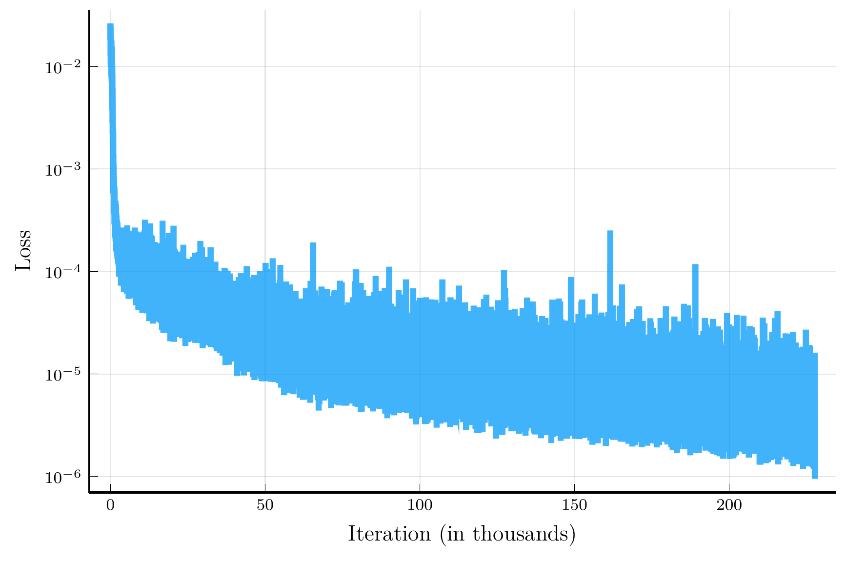

Loss history

Value function

A Q-theory of investment

Consider the case where there are no equity issuance costs, i.e., \(\lambda = 0\).

• In this case, the investment rate is given by the q-theory of investment: \(i(k,z) = \frac{v_k(k,z) - 1}{\chi}\).
• We will solve for the optimal investment without using the first-order condition explicitly.

In addition to a neural network for the value function, we will also use a neural network for the optimal investment policy.

i_core = Chain(
    Dense(2, 32, Lux.swish),
    Dense(32, 24, Lux.swish),
    Dense(24, 1)
)
i_net(s, θᵢ) = i_core(s, θᵢ, stᵢ)[1]

# Initialize the parameters and optimizer
rng                  = Xoshiro(1234)
θᵢ, stᵢ              = Lux.setup(rng, i_core) |> Lux.f64
optᵢ                 = Optimisers.Adam(1e-3)
osᵢ                  = Optimisers.setup(optᵢ, θᵢ)

Implementing the implicit version of policy evaluation

We will use the implicit version of policy evaluation:

\[ \mathbf{\theta}_V^{j} = \mathbf{\theta}_V^{j-1} - \eta_V \frac{1}{I}\sum_{i=1}^I HJB(\mathbf{s}_i, \mathbf{\theta}_C^{j}, \mathbf{\theta}_V^{j-1}) \nabla_{\mathbf{\theta}_V} HJB(\mathbf{s}_i, \mathbf{\theta}_C^{j}, \mathbf{\theta}_V^{j-1}), \]

The term \(\nabla_{\mathbf{\theta}_V} HJB(\mathbf{s}_i, \mathbf{\theta}_C^{j}, \mathbf{\theta}_V^{j-1})\) depends on the gradient and Hessian of the value function.

• Hence, this requires computing a third-order derivative of the value function.

• This type of mixed-mode automatic differentiation is not supported by many AD systems.

To overcome this challenge, we will use the hyper-dual approach to Itô’s lemma.

• This requires computing a second derivative of a univariate function.

  • With automatic differentiation, we would face the mixed-mode limitation.

• We will compute this second derivative using finite-differences.

  • This way, Zygote never interacts with dual numbers, and can differentiate the HJB residuals without difficulty.

The HJB residuals

First, we define a function that computes the second derivative of the value function using finite-differences.

• We consider the usual three-point stencil, but also include higher-order stencils as options.

function second_derivative_FD(F::Function, h::Float64; stencil::Symbol = :three)
    if stencil == :nine
        return (-9.0 .* F(-4h) .+ 128.0 .* F(-3h) .- 1008.0 .* F(-2h) .+ 8064.0 .* F(-h) .- 14350.0 .* F(0.0) .+ 8064.0 .* F(h) .- 1008.0 .* F(2h) .+ 128.0 .* F(3h) .- 9.0 .* F(4h)) ./ (5040.0 * h^2)
    elseif stencil == :seven
        return (2.0 .* F(-3h) .- 27.0 .* F(-2h) .+ 270.0 .* F(-h) .- 490.0 .* F(0.0) .+ 270.0 .* F(h) .- 27.0 .* F(2h) .+ 2.0 .* F(3h)) ./ (180.0 * h^2)
    elseif stencil == :five
        return (-F(2h) .+ 16.0 .* F(h) .- 30.0 .* F(0.0) .+ 16.0 .* F(-h) .- F(-2h)) ./ (12.0 * h^2)
    else 
        return (F(h) - 2.0 * F(0.0) + F(-h)) / (h*h) # Three point stencil
    end
end

Given this function, we can define the HJB residual.

function hjb_residual(m, s, θᵥ, θᵢ; h = 5e-2, stencil::Symbol = :three)
    (; α, λ, ρ, δ, χ) = m
    k, z   = s[1,:]', s[2,:]'
    i      = i_net(s, θᵢ)
    D_star = exp.(z) .* k.^α - (i + 0.5*χ*i.^2).*k
    D      = D_star .* (1 .+ λ * (D_star .< 0))
    μk     = (i .- δ) .* k
    μz     = -θ .* (z .- z̅)
    μₛ     = vcat(μk, μz)
    σₛ     = vcat(zeros(1, size(s,2)), σz*ones(1, size(s,2)))
    F(ϵ)   = v_net(s .+ σₛ .* (ϵ / sqrt(2.0)) .+ μₛ * (ϵ^2 / 2.0), θᵥ)
    drift  = second_derivative_FD(F, h, stencil = stencil)
    hjb    = D + drift - m.ρ * v_net(s, θᵥ)
    return hjb
end

Loss functions and training parameters

First, we define the loss functions for the value function

• In this formulation, we minimize directly the mean squared HJB residuals.

function loss_v(m, s, θᵥ, θᵢ; h = 5e-2, stencil::Symbol = :nine)
    hjb = hjb_residual(m, s, θᵥ, θᵢ; h = h, stencil = stencil)
    return mean(abs2, hjb)
end

Next, we define the loss function for the optimal investment policy.

• The loss corresponds to minus the mean HJB residuals, as we want to maximize the right-hand side of the HJB equation.

function loss_i(m, s, θᵥ, θᵢ; h = 5e-2, stencil::Symbol = :nine)
    hjb = hjb_residual(m, s, θᵥ, θᵢ; h = h, stencil = stencil)
    return -mean(hjb)
end

Finally, we define the training parameters.

max_iter             = 300_000
kmin, kmax           = 1.0, 8.0
dk                   = Uniform(kmin, kmax)
dz                   = Normal(m.z̅, m.σz/sqrt(2.0*m.θ))

Training loop

We can now define the training loop.

loss_history_v = Float64[];
loss_history_i = Float64[];
nsteps_v, nsteps_i = 10, 1
for it in 1:max_iter
    s_batch = vcat(rand(rng, dk, 150)', rand(rng, dz, 150)')
    lossᵥ, lossᵢ = zero(Float64), zero(Float64)
    # Policy evaluation step
    for _ = 1:nsteps_v
        lossᵥ, backᵥ = Zygote.pullback(p -> loss_v(m, s_batch, p, θᵢ), θᵥ)
        gradᵥ        = first(backᵥ(1.0))
        osᵥ, θᵥ      = Optimisers.update(osᵥ, θᵥ, gradᵥ)
    end
    # Policy improvement step
    for _ = 1:nsteps_i
        lossᵢ, backᵢ = Zygote.pullback(p -> loss_i(m, s_batch, θᵥ, p), θᵢ)
        gradᵢ        = first(backᵢ(1.0))
        osᵢ, θᵢ      = Optimisers.update(osᵢ, θᵢ, gradᵢ)
    end
    # Compute loss
    lossᵥ = loss_v(m, s_batch, θᵥ, θᵢ)
    lossᵢ = loss_i(m, s_batch, θᵥ, θᵢ)
    push!(loss_history_v, lossᵥ)
    push!(loss_history_i, lossᵢ)
    if max(lossᵥ, abs(lossᵢ)) < 1e-6
        println("Iteration ", it, "| Loss_v = ", lossᵥ, "| Loss_i = ", lossᵢ)
        break
    end
end

Training history and value function

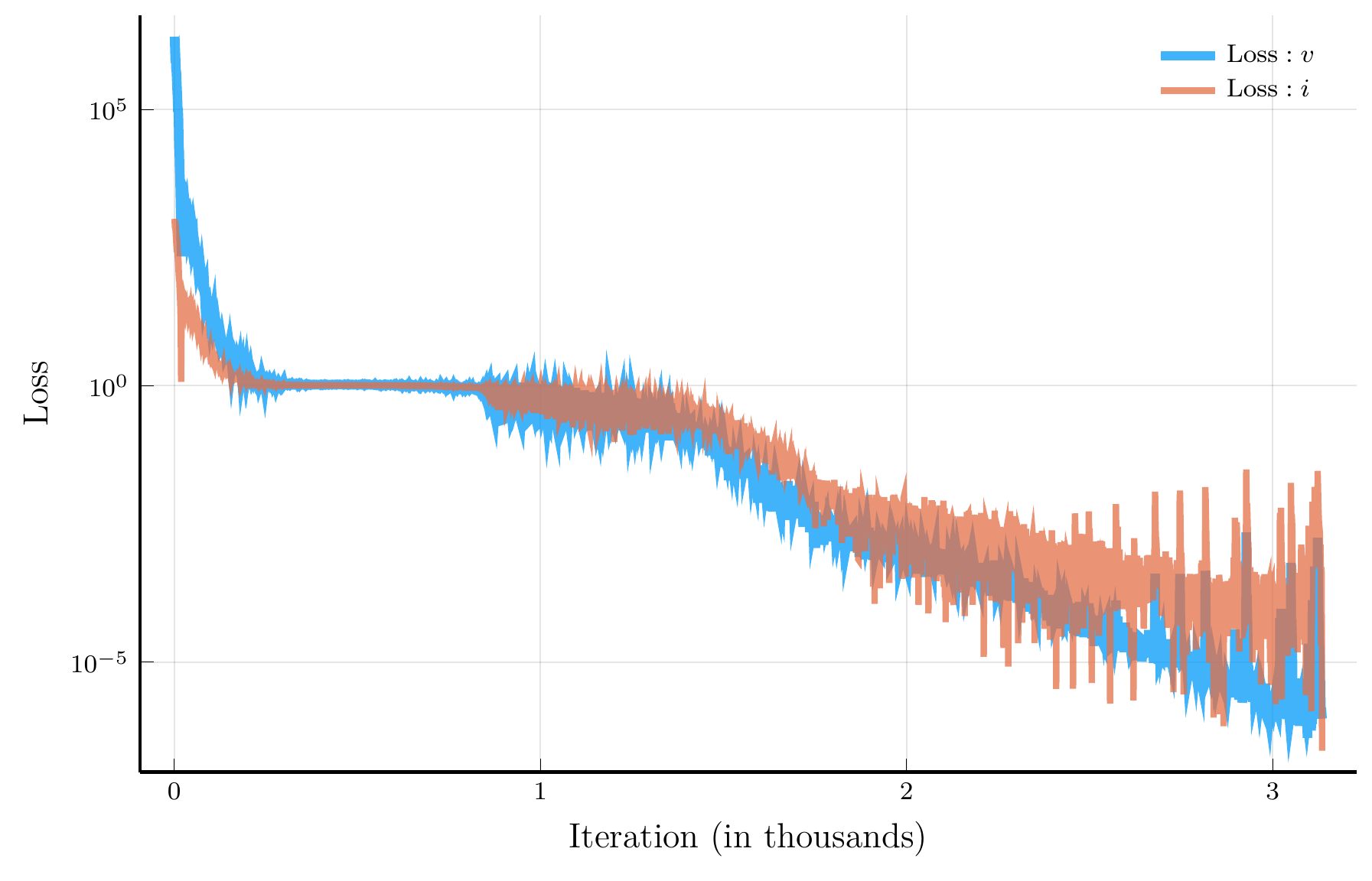
Loss history

Value function

Optimal Dividend Policy and Investment Rate

We consider next the optimal dividend policy and investment rate for the full model with \(\lambda > 0\).

• We compare the results with the finite-difference solution.

Dividends

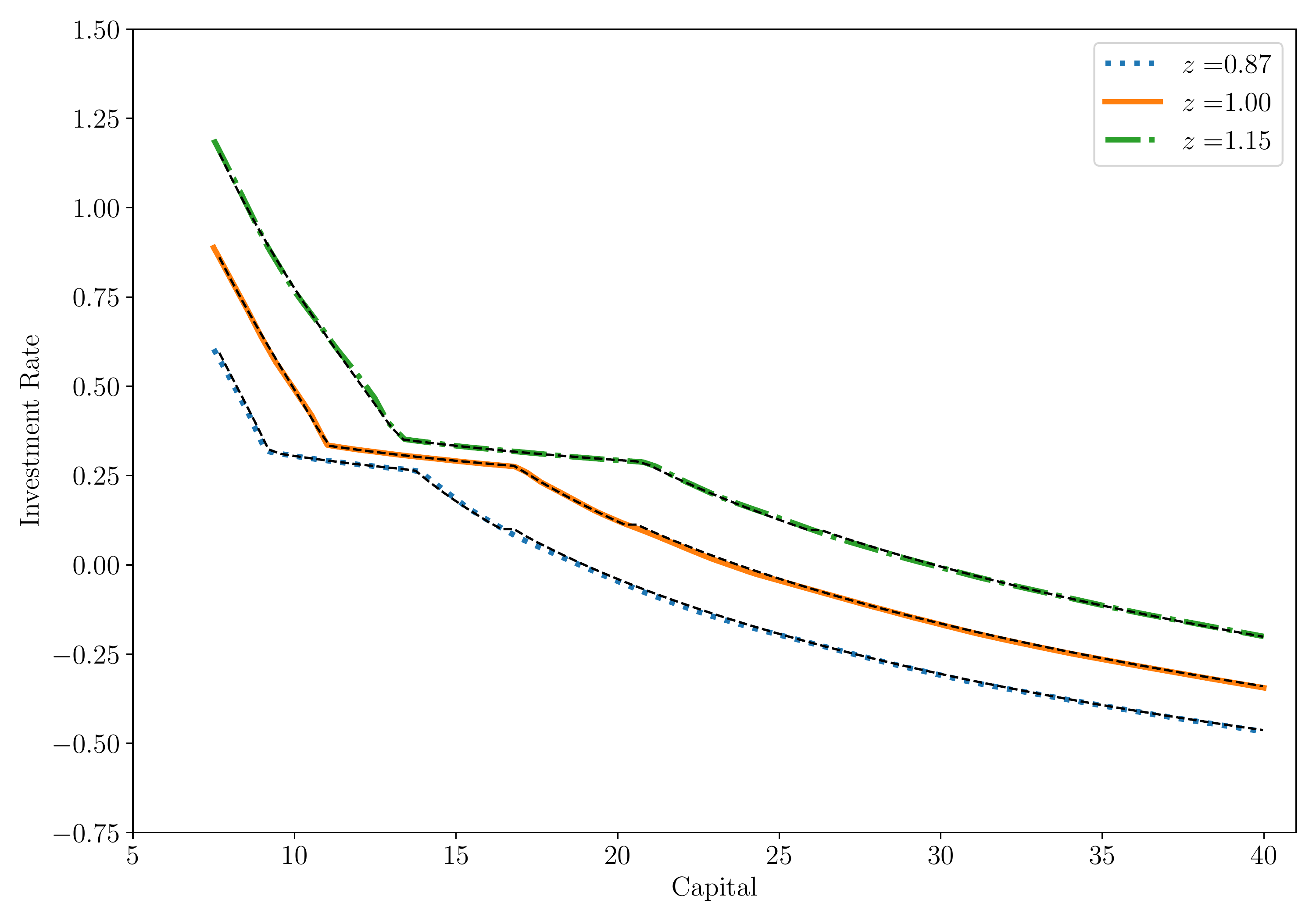
Investment Rate

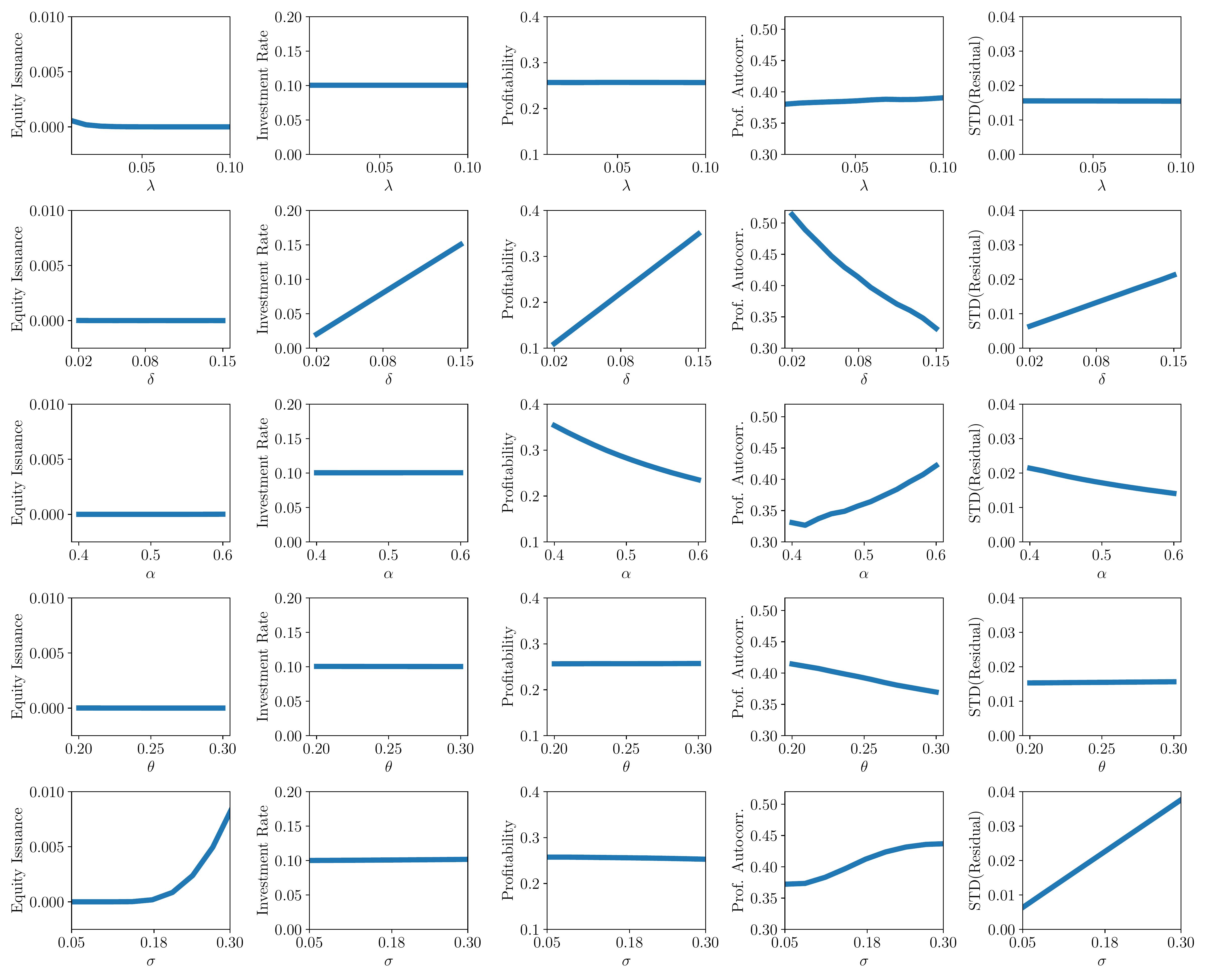
Global sensitivity analysis

This problem has only two state variables, so it can be easily solved using finite differences

• But we are often interested in the solution for a large number of parameter values
• For instance, how does the solution vary with investment or equity issuance costs?

In particular, we are interested in knowing which equilibrium moments are more sensitive to parameters

• This way we know which aspects of the data are more informative about the parameters
• To answer these questions, we need to perform a global sensitivity analysis

Performing such global sensitivity analysis can be computationally very costly

• Using the DPI method, we can overcome this challenge
• Solution: add the vector of parameters to the state space
• In deep-reinforcement learning, this is known as universal value functions

Global sensitivity analysis results

VI. Applications: Portfolio Choice

Portfolio Choice with Realistic Dynamics

As our third application, we consider a portfolio choice problem with realistic dynamics

• The problem will feature a large number of state variables, shocks, and controls

We consider the problem of an investor with Epstein-Zin preferences

• Investor must choose consumption and portfolio
• Investor has access to \(5\) risky assets and a risk-free asset

Volatility is constant and expected returns are affine functions of the state \(\mathbf{x}_t \in \mathbb{R}^n\)

• The state variable follows a multivariate Ornstein-Uhlenbeck (O-U) process: \[ d \mathbf{x}_t = - \Phi \mathbf{x}_t + \sigma_{\mathbf{x}} d \mathbf{B}_t, \]

To ensure absence of arbitrage, expected returns are derived from a state-price density (SPD)

• The price of risk and interest rate are affine functions of the state \[ r(\mathbf{x}_t) = r_0 + \mathbf{r}_1^{\top} \mathbf{x}_t, \qquad \qquad \boldsymbol{\eta}(\mathbf{x}_t) = \boldsymbol{\eta}_0 + \boldsymbol{\eta}_1^\top \mathbf{x}_t. \]

State variables

List of State Variables Driving the Expected Returns of Assets

Variable	Description	Mean	S.D. (%)
\(\pi_t\)	Log Inflation	0.032	2.3
\(y_t^{\$}(1)\)	Log 1-Year Nominal Yield	0.043	3.1
\(yspr_t^{\$}\)	Log 5-Year Minus 1-Year Nominal Yield Spread	0.006	0.7
\(\Delta z_t\)	Log Real GDP Growth	0.030	2.4
\(\Delta d_t\)	Log Stock Dividend-to-GDP Growth	-0.002	6.3
\(d_t\)	Log Stock Dividend-to-GDP Level	-0.270	30.5
\(pd_t\)	Log Stock Price-to-Dividend Ratio	3.537	42.6
\(\Delta\tau_t\)	Log Tax Revenue-to-GDP Growth	0.000	5
\(\tau_t\)	Log Tax Revenue-to-GDP Level	-1.739	6.5
\(\Delta g_t\)	Log Spending-to-GDP Growth	0.006	7.6
\(g_t\)	Log Spending-to-GDP Level	-1.749	12.9

Notes: The table shows the list of 11 state variables driving expected returns in our economy, along with their mean and standard deviation. The data are collected from https://www.publicdebtvaluation.com/data. See Jiang et al. (2024) for more details.

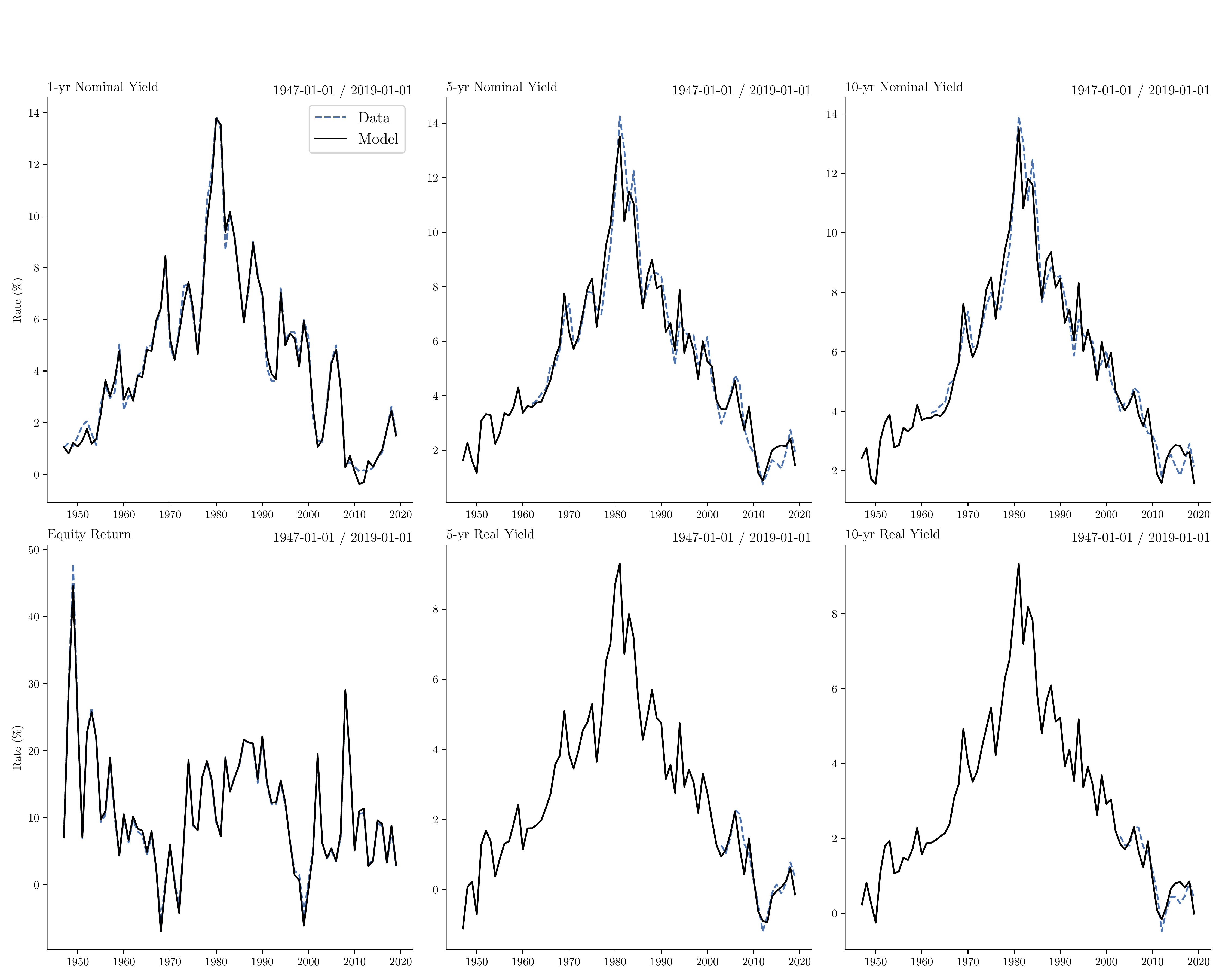
Estimation of continuous-time SPD

State dynamics estimation

• We run a discrete time VAR on the \(n = 11\) state variables: \[ \mathbf{x}_t = \Psi \mathbf{x}_{t-1} + \mathbf{u}_t. \]
• Find \(\Phi\) and \(\sigma_{\mathbf{x}}\) such that the time-integrated continuous-time process coincides with VAR

State-price density estimation

• Find \((r_0,\mathbf{r}_1,\boldsymbol{\eta}_0, \boldsymbol{\eta}_1)\) to minimize squared deviations of model-implied and data moments
• Moments: time-integrated time series for nominal yields, real yields, and expected stock returns

Bond Yields and Equity Expected Returns

Time Series of Expected Returns and Optimal Allocations

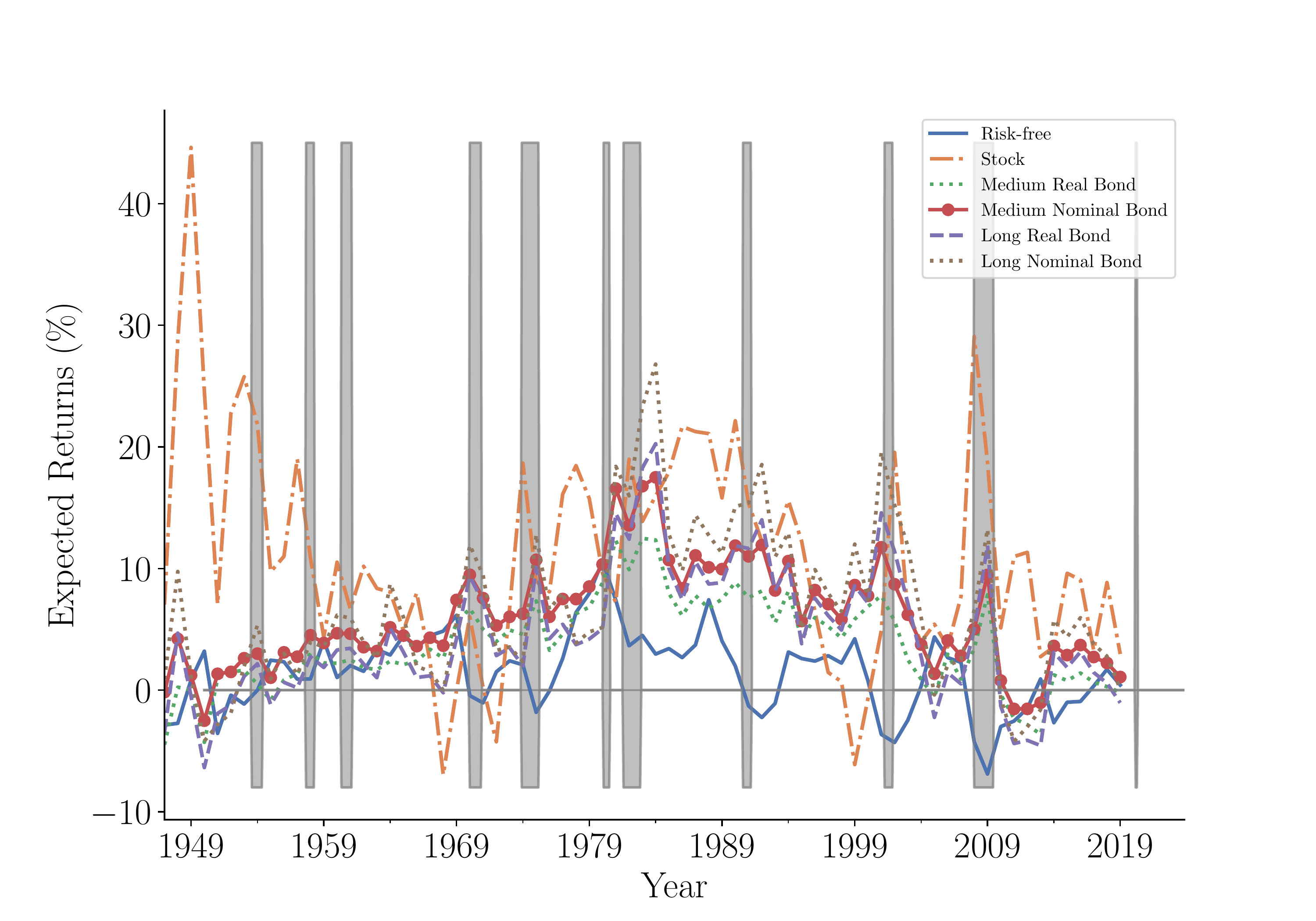
Expected Returns

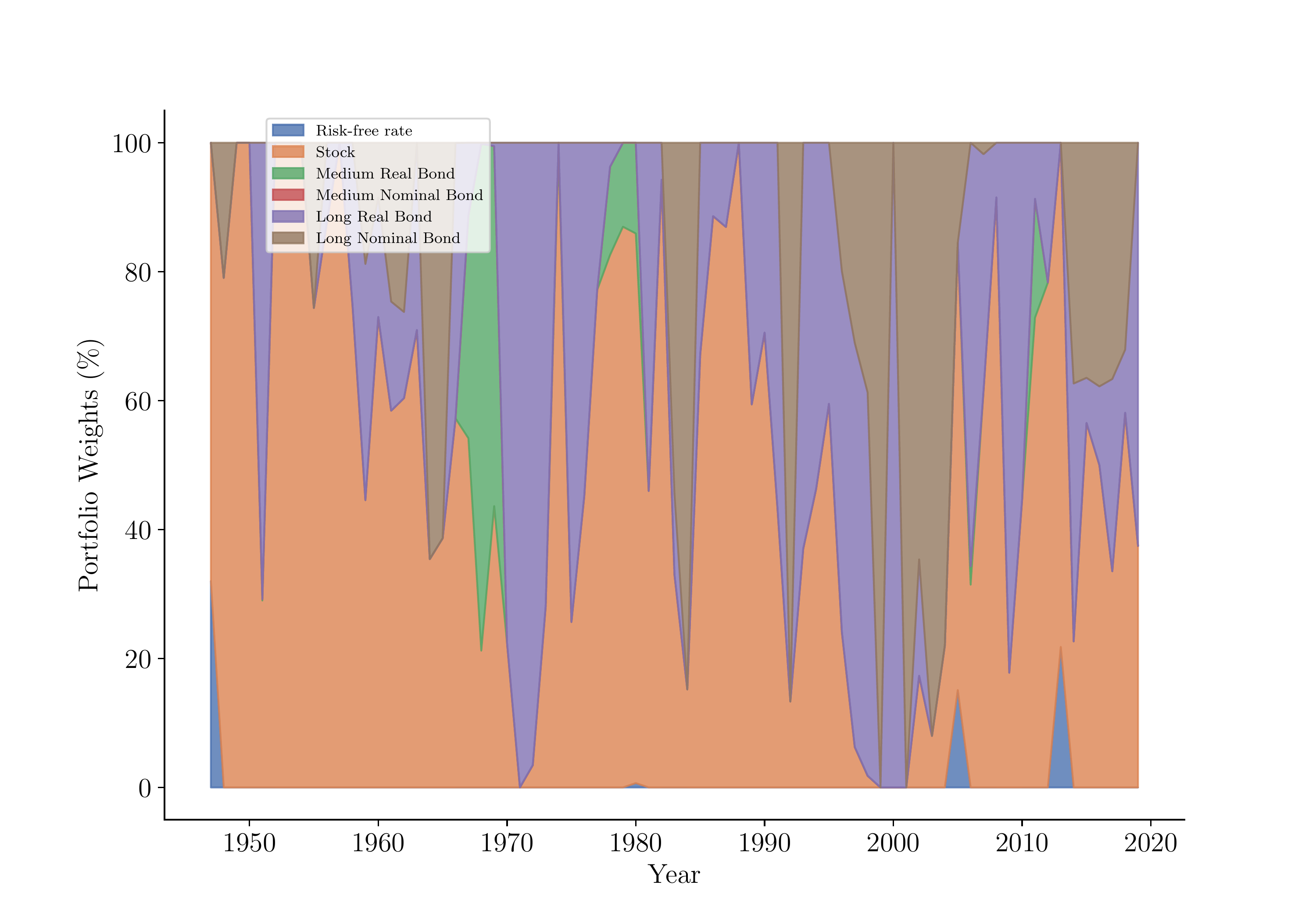
Asset Allocation

Optimal allocation

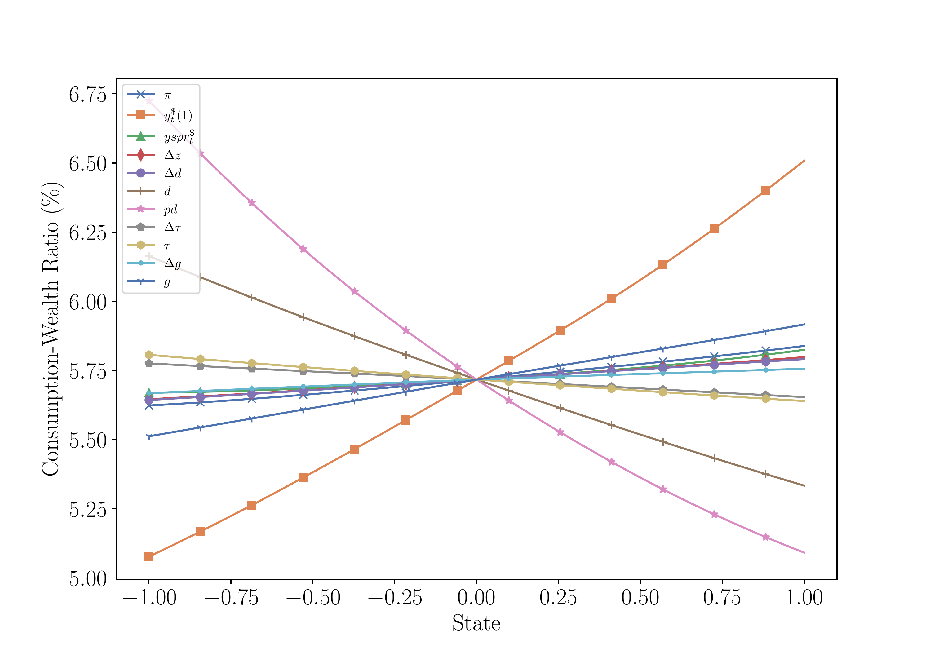
Consumption-Wealth Ratio

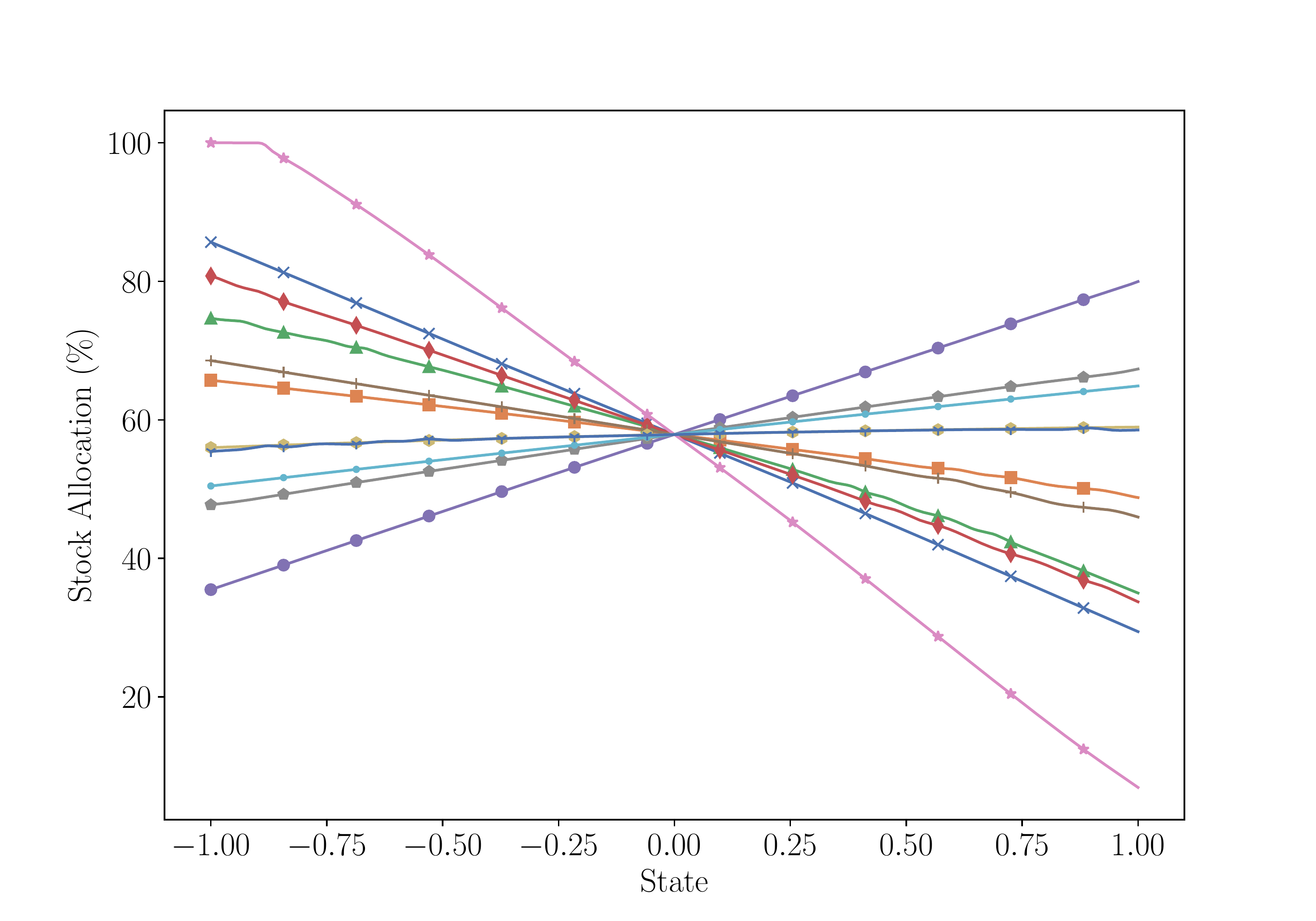
Stock

Optimal portfolio (continued)

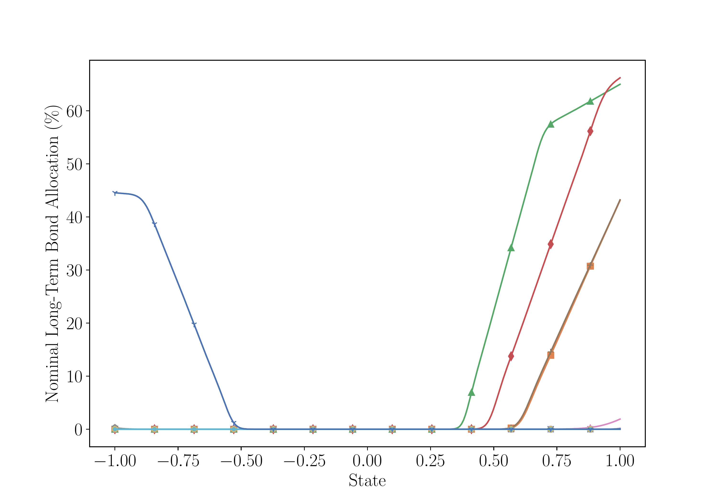
Nominal Long-Term Bond

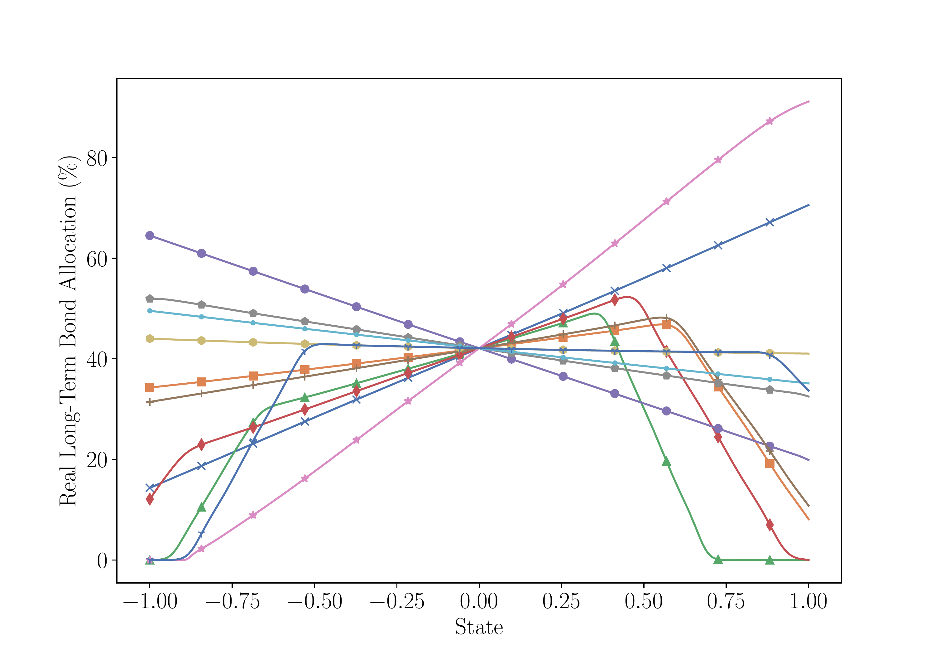
Real Long-Term Bond

Conclusion

In this lecture, we learned methods that alleviate the three curses of dimensionality

1. Use deep neural networks to represent \(V(\mathbf{s})\)
2. Compute expectations using Itô’s lemma and automatic differentiation
3. Gradient-based update rule that does not rely on root-finding procedures

The DPI algorithm allows us to solve high-dimensional problems

• Method is effective in situations where leading numerical methods fail

Ability to solve rich problems can be an invaluable tool in economic analysis

• We oftentimes make assumptions that have no clear economic interest
  • Assumptions are made only for tractability reasons
• Our method enables researchers to focus on economically interesting models
  • Instead of focusing on models that we could easily solve

References

Duarte, Victor, Diogo Duarte, and Dejanir H. Silva. 2024. “Machine Learning for Continuous-Time Finance.” The Review of Financial Studies 37 (11): 3217–71. https://doi.org/10.1093/rfs/hhae043.

Hennessy, Christopher A, and Toni M Whited. 2007. “How Costly Is External Financing? Evidence from a Structural Estimation.” Journal of Finance 62 (4): 1705–45.

Jiang, Zhengyang, Hanno Lustig, Stijn Van Nieuwerburgh, and Mindy Z. Xiaolan. 2024. “The u.s. Public Debt Valuation Puzzle.” Econometrica 92 (4): 1309–47. https://doi.org/10.3982/ECTA17674.

Martin, Ian. 2013. “The Lucas Orchard.” Econometrica 81 (1): 55–111. https://doi.org/10.3982/ECTA8446.

Smolyak, Sergei Abramovich. 1963. “Quadrature and Interpolation Formulas for Tensor Products of Certain Classes of Functions.” In Doklady Akademii Nauk, 148:1042–45. 5. Russian Academy of Sciences.

Sutton, Richard S., and Andrew G. Barto. 2018. Reinforcement Learning: An Introduction. 2nd ed. Cambridge, MA: MIT Press. http://incompleteideas.net/book/the-book-2nd.html.